In this blog, we’ll explore how to use a neural network built with PyTorch to predict handwritten digits from the MNIST dataset. Along the way, we’ll break down key concepts like tensors, neural network architecture, and training processes, making it easier to understand the fundamental building blocks of deep learning.

The MNIST dataset, a collection of 28x28 grayscale images of digits (0–9), is a classic benchmark for machine learning. Our goal is to create a model that accurately recognizes these digits using the power of neural networks.

Introduction

Machine learning is a transformative tool for modeling complex relationships in data. Neural networks, a class of machine learning models inspired by the human brain, are particularly adept at handling non-linear relationships. This post explores their application, focusing on tensors, neural networks, and their underlying theory.

Tensors: The Backbone of Neural Networks

At the heart of neural networks lie tensors, multidimensional arrays that generalize matrices to higher dimensions. They efficiently handle complex data like images, text, or time series, making them critical for machine learning.

For instance, a scalar is a rank-0 tensor (a single number), a vector is rank-1 (a sequence of numbers), and a matrix is rank-2 (a 2D grid). Consider This 2D input tensor x, which could represent a dataset:

import torch 
x = torch.tensor([[1, 2], [3, 4], [5, 6]])  # A 2D tensor (matrix)
print(x)

## tensor([[1, 2],
##         [3, 4],
##         [5, 6]])

Tensors flow through the network, undergoing operations like matrix multiplication and activation functions, ultimately producing outputs. Their ability to efficiently process data on GPUs makes tensors indispensable for modern machine learning.

Neural Network Architecture

A neural network is composed of layers of interconnected nodes (neurons) that process input data and produce predictions:

• Input Layer: Receives the raw data (e.g., tensors representing images, text, or numbers) and passes it to the next layer.
• Hidden Layers: These intermediate layers perform computations, applying weights, biases, and activation functions to extract meaningful patterns and features.
• Output Layer: Generates the final output, such as classifications, predictions, or probabilities.

Each connection between neurons has a weight that adjusts during training, enabling the network to learn from data by minimizing error. Activation functions like ReLU or Sigmoid introduce non-linearity, allowing the network to model complex relationships.

Example Model Configuration

The neural network model in this example uses a simple feedforward architecture. We define it as:

import torch.nn as nn

class SimpleNN(nn.Module):
    def __init__(self, input_size, hidden_size, output_size):
        super(SimpleNN, self).__init__()
        self.fc1 = nn.Linear(input_size, hidden_size)
        self.relu = nn.ReLU()
        self.fc2 = nn.Linear(hidden_size, output_size)
    
    def forward(self, x):
        x = self.fc1(x)
        x = self.relu(x)
        x = self.fc2(x)
        return x

input_size = 28 * 28  # Example: 28x28 images
hidden_size = 128
output_size = 10  # Example: 10 classes

model = SimpleNN(input_size, hidden_size, output_size)

Lets dive into a more detailed code explanation of the neural network architecture.

1. The Dataset: MNIST

The MNIST dataset is a collection of grayscale images of handwritten digits, commonly used as a benchmark dataset in machine learning. Each image is:

• 28x28 pixels in size.
• Labeled with a number from 0 to 9 (10 classes in total).

Code Explanation

from torchvision import datasets, transforms

# Define transformations for the dataset
transform = transforms.Compose([transforms.ToTensor()])

• Transforms: The dataset is preprocessed using transforms.ToTensor(), which converts the images into PyTorch tensors (normalized to [0, 1]).
• Compose: Allows multiple transformations to be chained together. Here, only the conversion to a tensor is applied.

# Load training and testing datasets
train_dataset = datasets.MNIST(root='./data', train=True, transform=transform, download=True)
test_dataset = datasets.MNIST(root='./data', train=False, transform=transform, download=True)

• train=True/False: Indicates whether to load the training or testing split of the MNIST dataset.

# Create DataLoaders
train_loader = DataLoader(train_dataset, batch_size=100, shuffle=True)
test_loader = DataLoader(test_dataset, batch_size=100, shuffle=False)

• DataLoader: A utility that:
  • Loads data in batches (size batch_size=100 here).
  • Shuffles the training data for randomness.
  • Ensures efficient data loading during training/testing.

A batch refers to a subset of the dataset processed at one time during training or inference. Instead of feeding the entire dataset to the model, which can be computationally expensive and memory-intensive, the data is divided into smaller groups (batches). Each batch passes through the network, computes predictions, and calculates the loss. The model then updates its weights based on the average loss of the batch. This approach balances efficiency and learning, making training manageable even for large datasets like MNIST.

2. The Neural Network: SimpleNN

A neural network is composed of layers of interconnected nodes (neurons) that process input data and produce predictions. Here’s how SimpleNN is structured:

Code Explanation

class SimpleNN(nn.Module):
    def __init__(self, input_size, hidden_size, output_size):
        super(SimpleNN, self).__init__()
        self.fc1 = nn.Linear(input_size, hidden_size)
        self.relu = nn.ReLU()
        self.fc2 = nn.Linear(hidden_size, output_size)

• nn.Module: Base class for all PyTorch models.
• __init__: Defines the structure of the neural network.
  • input_size: The number of input features (28x28 = 784 for MNIST images flattened into vectors).
  • hidden_size: Number of neurons in the hidden layer (set to 128 here).
  • output_size: The number of output classes (10 digits: 0 to 9).
  • fc1: A fully connected (dense) layer that transforms the input into the hidden layer with dimensions [input_size -> hidden_size].
  • ReLU: Applies the ReLU activation function, introducing non-linearity to the model. ReLU replaces negative values with 0.
  • fc2: A fully connected layer that transforms the hidden layer output to the final output layer with dimensions [hidden_size -> output_size].

    def forward(self, x):
        x = self.fc1(x)
        x = self.relu(x)
        x = self.fc2(x)
        return x

• forward: Defines how data flows through the network.

1. Passes the input through fc1 (input layer).
2. Applies the ReLU activation.
3. Passes the result through fc2 (output layer).
4. Returns the final output.

init establishes the components of the network, and forward dictates how those components are used during the forward pass. Together, they form the blueprint and operational flow of the model.

The ReLU activation function (Rectified Linear Unit) is one of the most commonly used activation functions in neural networks, especially in deep learning. Its popularity stems from its simplicity, efficiency, and effectiveness.

What Is ReLU?

The ReLU function is defined mathematically as:

$$ f(x) = \begin{cases} x & \text{if } x > 0 \\
0 & \text{if } x \leq 0 \end{cases} $$ Or simply:

$$ f(x) = \max(0, x) $$ In words, ReLU outputs the input value directly if it’s positive and outputs 0 for any negative value.

Why Use an Activation Function?

Activation functions introduce non-linearity into the neural network. Without an activation function, the network would simply consist of linear transformations (matrix multiplications), which means it would only be able to model linear relationships in data. Non-linear activation functions, like ReLU, allow the network to model complex, non-linear relationships.

ReLU is applied to the output of each neuron (or unit) in a layer after the weighted sum of inputs and bias. Here’s what happens:

1. A neuron calculates a weighted sum of its inputs:

$$ z = \mathbf{w} \cdot \mathbf{x} + b, \\ \
where: \\ \
\mathbf{w}: Weights, \\ \
\mathbf{x}: Inputs, \\ \
b: Bias $$

2. The ReLU function is applied to (z) to produce the neuron’s output:

$$a = f(z) = \max(0, z)$$

This process is repeated across all neurons in the layer.

Benefits of ReLU

1. Simplicity: ReLU is computationally inexpensive because it involves simple thresholding at zero. Unlike other activation functions, like sigmoid or tanh, it does not require complex mathematical operations like exponentials.
2. Avoids Vanishing Gradients:
   • Activation functions like sigmoid and tanh compress outputs into a small range, which can cause gradients to vanish during backpropagation, making learning very slow in deep networks.
   • ReLU doesn’t compress values, so the gradient is preserved for positive inputs, enabling faster and more stable learning.
3. Efficient Sparsity:
   • Since ReLU outputs 0 for negative inputs, it introduces sparsity in the network. Sparsity helps by reducing the dependency between neurons and improving computation efficiency.

• ReLU introduces non-linearity between the input and output layers, allowing the network to learn complex patterns in the MNIST dataset.
• Its simplicity and efficiency make it an ideal choice for a small-scale network like this one.

Visualizing ReLU

Here’s how ReLU behaves visually:

• For $(x > 0)$, ReLU outputs the same value.
• For $(x \leq 0)$, ReLU outputs 0.

In summary, ReLU is simple, fast, and effective for training deep neural networks, making it the default choice in many modern architectures.

3. Model Initialization

input_size = 28 * 28  # Example: 28x28 images
hidden_size = 128
output_size = 10  # Example: 10 classes

model = SimpleNN(input_size, hidden_size, output_size)

• input_size = 28 * 28: Each MNIST image is a 28x28 matrix. Before feeding it into the model, it’s flattened into a 1D tensor of size 784.
• hidden_size = 128: The hidden layer contains 128 neurons. This is a hyperparameter and can be adjusted.
• output_size = 10: The output layer contains 10 neurons, one for each digit class (0 to 9).
• model: Instantiates the SimpleNN class with the specified parameters.

4. Model Training Expectations

The goal is to train the model to correctly classify MNIST digits with high accuracy. Here’s what we expect:

• Input: A batch of flattened MNIST images ([batch_size, 784]).
• Hidden Layer: Maps the input to a feature space of size 128.
• Output Layer: Produces probabilities for each digit class using a softmax layer (applied externally during training).
• Loss Function: Measures how far the predictions are from the true labels.
• Optimization: Uses Stochastic Gradient Descent (SGD) or another optimizer to minimize the loss by adjusting weights.

The loss function serves as a key metric in machine learning, quantifying how well or poorly a model’s predictions align with the actual target values. By evaluating the difference between the predicted outcomes and the true labels, the loss function provides a numerical value that guides the optimization process, helping to improve the model’s performance.

To minimize this loss, gradient descent is often used as an optimization algorithm. It works by iteratively adjusting the model’s parameters in the direction that reduces the loss function the most. By following the gradient (or slope) of the loss function, gradient descent ensures the model progressively improves its predictions, moving closer to the optimal solution.

5. Expected Results

• Accuracy: For a simple feedforward network like this, we expect around 90%-92% accuracy on the MNIST test set after training.
• Loss: The loss will start high (e.g., 2.0) and gradually decrease to values around 0.3-0.5 as the model learns.
• Improvement Potential:
  • Adding more hidden layers or increasing the hidden size.
  • Experimenting with advanced architectures like CNNs.
  • Using data augmentation techniques for better generalization.

Example

Lets combine this concepts, and run the model in order the get the results.

Data Loading

We use PyTorch’s DataLoader to load the training and testing data.

from torch.utils.data import DataLoader
from torchvision import datasets, transforms

# Define transformations for the dataset
transform = transforms.Compose([transforms.ToTensor()])

# Load training and testing datasets
train_dataset = datasets.MNIST(root='./data', train=True, transform=transform, download=True)
test_dataset = datasets.MNIST(root='./data', train=False, transform=transform, download=True)

# Create DataLoaders
train_loader = DataLoader(train_dataset, batch_size=100, shuffle=True)
test_loader = DataLoader(test_dataset, batch_size=100, shuffle=False)

Loss Function and Optimizer

We use Cross Entropy Loss as the loss function and SGD as the optimizer:

import torch.optim as optim

loss_fn = nn.CrossEntropyLoss()
optimizer = optim.SGD(model.parameters(), lr=0.01)

Training the Neural Network

Training a neural network involves repeatedly feeding data through the model, calculating the error (loss), and updating the model’s parameters using optimization techniques like gradient descent. The train_loop() function handles this process for each training epoch.

Here’s how train_loop() is implemented:

def train_loop(dataloader, model, loss_fn, optimizer):
    """
    Training loop for a neural network model.
    
    Parameters:
    - dataloader: DataLoader object for training data
    - model: Neural network model
    - loss_fn: Loss function (e.g., CrossEntropyLoss)
    - optimizer: Optimizer (e.g., SGD, Adam)

    Returns:
    None
    """
    size = len(dataloader.dataset)
    model.train()
    
    for batch, (X, y) in enumerate(dataloader):
        # Flatten images into vectors
        X = X.view(X.size(0), -1)
        
        # Forward pass
        pred = model(X)
        loss = loss_fn(pred, y)
        
        # Backpropagation
        optimizer.zero_grad()
        loss.backward()
        optimizer.step()
        
        # Log progress
        if batch % 100 == 0:
            loss_current = loss.item()
            print(f"loss: {loss_current:>7f}  [{batch * len(X):>5d}/{size:>5d}]")

This function is executed within each training epoch, as shown below:

for epoch in range(5):
    train_loop(train_loader, model, loss_fn, optimizer)

## loss: 2.302421  [    0/60000]
## loss: 2.082567  [10000/60000]
## loss: 1.820236  [20000/60000]
## loss: 1.481050  [30000/60000]
## loss: 1.281981  [40000/60000]
## loss: 1.009585  [50000/60000]
## loss: 0.945703  [    0/60000]
## loss: 0.837330  [10000/60000]
## loss: 0.799911  [20000/60000]
## loss: 0.746439  [30000/60000]
## loss: 0.629169  [40000/60000]
## loss: 0.529109  [50000/60000]
## loss: 0.390061  [    0/60000]
## loss: 0.420087  [10000/60000]
## loss: 0.353291  [20000/60000]
## loss: 0.467722  [30000/60000]
## loss: 0.710849  [40000/60000]
## loss: 0.349696  [50000/60000]
## loss: 0.385319  [    0/60000]
## loss: 0.443223  [10000/60000]
## loss: 0.247738  [20000/60000]
## loss: 0.438087  [30000/60000]
## loss: 0.547100  [40000/60000]
## loss: 0.468050  [50000/60000]
## loss: 0.330704  [    0/60000]
## loss: 0.365649  [10000/60000]
## loss: 0.326305  [20000/60000]
## loss: 0.363884  [30000/60000]
## loss: 0.315488  [40000/60000]
## loss: 0.360471  [50000/60000]

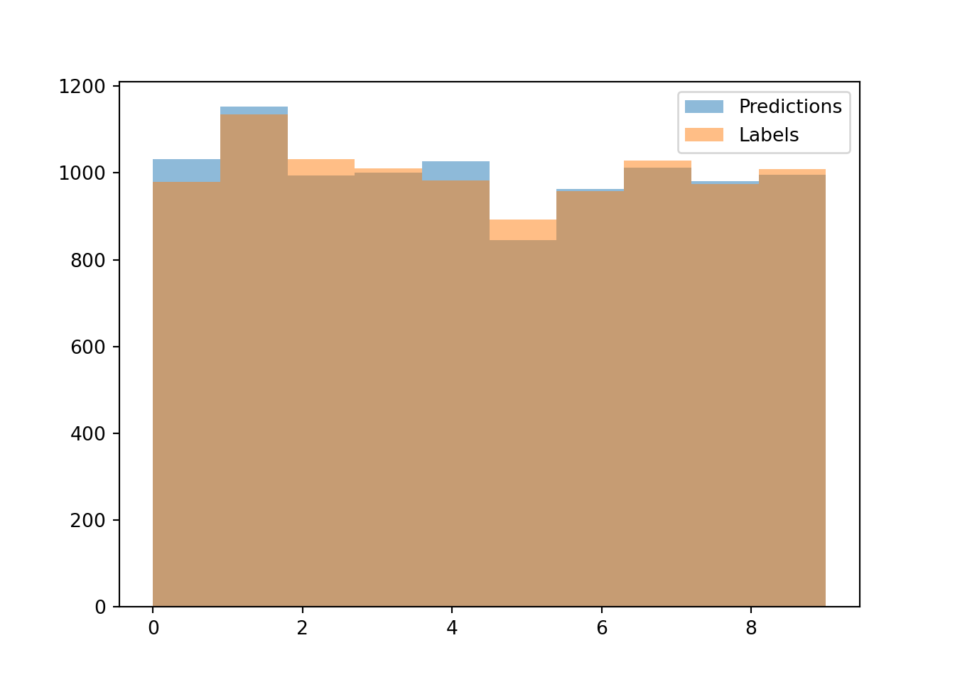
Visualizing Predictions

After training, we can compare the model’s predictions to true labels using a histogram:

import matplotlib.pyplot as plt

def test_loop(dataloader, model, loss_fn):
    model.eval()
    size = len(dataloader.dataset)
    num_batches = len(dataloader)
    test_loss = 0
    correct = 0
    all_preds = []
    all_labels = []
    
    with torch.no_grad():
        for X, y in dataloader:
            X = X.view(X.size(0), -1)
            pred = model(X)
            test_loss += loss_fn(pred, y).item()
            correct += (pred.argmax(1) == y).type(torch.float).sum().item()
            all_preds.extend(pred.argmax(1).tolist())
            all_labels.extend(y.tolist())
    
    test_loss /= num_batches
    correct /= size
    return test_loss, correct, all_preds, all_labels

test_loss, test_acc, pred, lab = test_loop(test_loader, model, loss_fn)
print(f"Test Error: \n Accuracy: {(100*test_acc):>0.1f}%, Avg loss: {test_loss:>8f} \n")

## Test Error: 
##  Accuracy: 90.5%, Avg loss: 0.341179

# Plot histograms
plt.hist(pred, bins=10, alpha=0.5, label='Predictions')
plt.hist(lab, bins=10, alpha=0.5, label='Labels')
plt.legend()
plt.show()

Conclusion

In this project, we trained a simple feedforward neural network on the MNIST dataset and evaluated its performance. The final results were as follows:

• Test Accuracy: 90.4%
• Average Test Loss: 0.3445

The histogram above shows that the predictions closely match the true labels, demonstrating that the neural network successfully learned patterns in the data. While the accuracy indicates solid performance, further improvements could be achieved through:

• Optimizing hyperparameters (e.g., learning rate, batch size, number of hidden units).
• Experimenting with deeper or more complex architectures like Convolutional Neural Networks (CNNs).
• Increasing the number of training epochs to allow the network to converge better.

This blog demonstrated how to build, train, and evaluate a simple feedforward neural network using PyTorch to classify handwritten digits from the MNIST dataset. Along the way, we covered essential concepts such as tensors, neural network architecture, activation functions, and the training process.

Neural networks are versatile tools with applications across diverse domains. This project serves as a foundation for understanding how to implement and optimize these models, paving the way for tackling more complex machine learning challenges in the future.

References

• PyTorch Documentation: https://pytorch.org/docs/
• MNIST Dataset: http://yann.lecun.com/exdb/mnist/