Analyzing Bitcoin Options with Deribit API and Black-Scholes Model

Introduction

Bitcoin options have become an essential tool in modern financial markets, offering traders and researchers opportunities to manage risk, speculate on price movements, and explore market dynamics. However, understanding and leveraging these instruments require a combination of financial knowledge and technical expertise.

This blog aims to provide a step-by-step guide to analyzing Bitcoin options by integrating key financial concepts with practical coding implementations. Specifically, we will:

1. Download and Process Historical Data:
   • Learn how to use the Deribit API to retrieve detailed Bitcoin options data, overcoming common challenges in data collection through Python automation.blog
2. Understand the Black-Scholes Model:
   • Explore the mathematical foundations of options pricing, focusing on how variables like volatility and time-to-maturity influence option values.
3. Apply Machine Learning for Volatility Forecasting:
   • Use a Random Forest model to predict implied volatility, showcasing a modern, data-driven approach to financial analysis.
4. Implement a Delta Strategy:
   • Discover how delta, a key measure in options trading, can be used to adjust portfolios dynamically and manage risk effectively.

We will be showing:

• API expertise: Using Python to interact with APIs and process large datasets effectively.
• Finance Foundations: Applying theoretical models like Black-Scholes in real-world scenarios.
• Machine Learning: Leveraging data-driven approaches to forecast critical metrics in financial markets.
• Strategic Thinking: Translating insights from data into actionable strategies, like delta crypto finance strategies

Part 1: Downloading Historical Bitcoin Options Data

We will use Deribit’s historical API to access Bitcoin options data. This API allows fetching complete historical data for options trades.

The standard Deribit API imposes a limitation on accessing historical data, allowing users to retrieve trades only up to two weeks in the past. To overcome this, Deribit provides a separate historical API endpoint, enabling access to older trade data with detailed records of options activity.

The steps involve setting up a loop to retrieve data in manageable time intervals and processing the results for further analysis.

Code Implementation:

import requests
import pandas as pd
from datetime import datetime, timedelta
import time

# Define the historical trades URL
historical_trades_url = "https://history.deribit.com/api/v2/public/get_last_trades_by_currency_and_time"

# Function to get historical trades
def get_historical_trades(currency, kind, start_time, end_time, count=1000):
    # Convert timestamps to milliseconds since epoch
    end_timestamp = int(time.mktime(end_time.timetuple()) * 1000)
    start_timestamp = int(time.mktime(start_time.timetuple()) * 1000)

    # Define the payload for fetching historical trades
    trades_payload = {
        'currency': currency,
        'start_timestamp': start_timestamp,
        'end_timestamp': end_timestamp,
        'kind': kind,
        'count': count,
        'include_old': True
    }

    # Send the request to get historical trades
    trades_response = requests.get(historical_trades_url, params=trades_payload)

    # Check if the response is successful
    if trades_response.status_code == 200:
        trades_data = trades_response.json()
        #print("Historical Trades Response:", trades_data)

        # Process and print trades data
        if 'result' in trades_data:
            print("Successfully fetched trades data")
        else:
            print("Failed to fetch trades data")
    else:
        print(f"Failed to fetch data: {trades_response.status_code}")
    return trades_data

# Function to process and filter trades data
def get_trades(trades_data):
    trades = trades_data['result']['trades']
    df = pd.json_normalize(trades)
    if 'timestamp' in df.columns:
        df['timestamp'] = pd.to_datetime(df['timestamp'], unit='ms')
        # Filter for call options
        calls = df[df['instrument_name'].str.endswith('C')].copy()
        # Extract maturity and strike prices
        calls.loc[:, 'maturity'] = calls['instrument_name'].apply(lambda x: x.split('-')[1])
        calls.loc[:, 'strike'] = calls['instrument_name'].apply(lambda x: x.split('-')[2].replace('C', '').replace('P', ''))
        calls['strike'] = calls['strike'].astype(float)

        calls['maturity'] = pd.to_datetime(calls['maturity'], format='%d%b%y')
        

    else:
       # print("No timestamp column for date", start_time)
        calls = pd.DataFrame()
    return calls

# Loop to fetch data for multiple time intervals
historical_trades = []
start_time = datetime(2024, 11, 7)  # Define starting time
for i in range(12):  # Loop to get data for 24 hours
    end_time = start_time + timedelta(hours=1)
    trades_response = get_historical_trades('BTC', 'option', start_time, end_time)
    historical_trades.append(get_trades(trades_response))
    start_time = end_time
    time.sleep(3)  # Wait 3 seconds between API calls

## Successfully fetched trades data
## Successfully fetched trades data
## Successfully fetched trades data
## Successfully fetched trades data
## Successfully fetched trades data
## Successfully fetched trades data
## Successfully fetched trades data
## Successfully fetched trades data
## Successfully fetched trades data
## Successfully fetched trades data
## Successfully fetched trades data
## Successfully fetched trades data

    
historical_trades = pd.concat(historical_trades, ignore_index=True)
print(historical_trades.head())

##    trade_seq   trade_id  ... combo_trade_id  liquidation
## 0        679  324402707  ...            NaN          NaN
## 1         43  324402703  ...            NaN          NaN
## 2         30  324402702  ...            NaN          NaN
## 3        678  324402688  ...            NaN          NaN
## 4       4318  324402676  ...            NaN          NaN
## 
## [5 rows x 18 columns]

Here’s a detailed explanation of what happens step by step:

Connecting to Deribit’s Historical API

The script interacts with the Deribit historical API endpoint, which allows fetching trade data for Bitcoin options. To use this API effectively, the script sends a structured request containing details such as the time range for the data, the type of instrument (e.g., options), and the currency (Bitcoin).

Data Retrieval in Time Intervals

Since the historical database can be extensive, the script divides the data request into manageable chunks. Specifically, it retrieves data in 1-hour intervals, starting from a defined start_time. This approach ensures that the API isn’t overwhelmed by large requests and adheres to any rate limits imposed by the server. After each request, the script waits for a few seconds before proceeding to the next, ensuring smooth communication with the API.

Filtering and Processing the Data

Once the trade data is retrieved, it is processed to extract relevant information. The script focuses on “call options,” a specific type of option contract, by filtering instruments whose names end with “C.” It further extracts important details such as:

• Strike Price: The agreed price at which the option can be exercised.
• Maturity Date: The expiration date of the option.

Automating the Workflow

To handle larger datasets, the script automates the entire workflow using a loop. For each iteration, it fetches data for a 1-hour window, processes the retrieved trades, and appends the results to a list. This list represents a cumulative collection of all the data retrieved across the defined time period (e.g., 7 hours in this example).

In summary:

1. Historical API: The URL https://history.deribit.com/api/v2/public/get_last_trades_by_currency_and_time allows accessing historical options data. Unlike the WebSocket API, this endpoint provides complete historical data.
2. Data Retrieval Loop: To avoid overwhelming the server, we query data in 1-hour intervals with a delay between requests.
3. Filtering and Processing:
   • Filters trades to extract only call options (instrument_name ends with C).
   • Extracts additional details like strike prices and maturity dates for analysis.

This code ensures efficient fetching of historical Bitcoin options data while adhering to API rate limits and provides well-structured data ready for modeling and analysis.

Part 2: Understanding the Black-Scholes Model

The Black-Scholes model is a mathematical formula for pricing European call and put options. It assumes constant volatility and no dividends.

Essentially, it determines the fair value of a call or put option based on several key factors: the current price of the underlying asset ($S_0$), the option’s strike price ($K$), the time left until expiration ($T$), the risk-free interest rate ($r$), and the volatility of the asset’s price ($ \sigma $). These variables are combined into a formula that accounts for the probabilistic nature of market movements and the time value of money.

At its core, the model calculates the likelihood of an option finishing “in the money” (profitable) by using two probability factors, $N(d_1)$ and $N(d_2)$, derived from the normal distribution. These terms represent the probabilities of different market scenarios. For a call option, the formula calculates the expected payoff by weighing the probability of the stock exceeding the strike price at expiration against the present value of the strike price itself. This balance ensures that the price reflects both the potential reward and the risks involved.

One of the key strengths of the Black-Scholes model is its simplicity and assumptions, such as constant volatility and no dividends. While these assumptions don’t always perfectly match reality, the model is an essential starting point for understanding option pricing and has paved the way for more advanced variations used in modern finance.

Formula:

The price of a call option is given by: $$ C = S_0 \cdot N(d_1) - K \cdot e^{-rT} \cdot N(d_2) $$ Where:

• $ S_0 $: Current stock price
• $ K $: Strike price
• $ T $: Time to expiration
• $ r $: Risk-free interest rate
• $ N(d) $: Cumulative standard normal distribution
• $ d_1 $: $ \frac{\ln(S_0 / K) + (r + \sigma^2 / 2)T}{\sigma \sqrt{T}} $
• $ d_2 $: $d_1 - \sigma \sqrt{T}$

Code:

from scipy.stats import norm
import numpy as np

# Black-Scholes Formula
def black_scholes(S, K, T, r, sigma, option_type="call"):
    d1 = (np.log(S / K) + (r + 0.5 * sigma ** 2) * T) / (sigma * np.sqrt(T))
    d2 = d1 - sigma * np.sqrt(T)
    if option_type == "call":
        return S * norm.cdf(d1) - K * np.exp(-r * T) * norm.cdf(d2)
    elif option_type == "put":
        return K * np.exp(-r * T) * norm.cdf(-d2) - S * norm.cdf(-d1)

# Example usage
S = 20000  # Current BTC price
K = 21000  # Strike price
T = 30 / 365  # Time to expiration in years
r = 0.01  # Risk-free rate
sigma = 0.5  # Volatility

call_price = black_scholes(S, K, T, r, sigma)
print(f"Call Option Price: {call_price}, for Strike Price: {K} and Time to Expiration: {T} years")

## Call Option Price: 744.2789814617408, for Strike Price: 21000 and Time to Expiration: 0.0821917808219178 years

Implied Volatility

Implied volatility (IV) is a measure of the market’s expectation of the future volatility of the underlying asset’s price. Unlike historical volatility, which is based on past price movements, IV is derived from the market price of options using models like Black-Scholes. It reflects the degree of expected price fluctuations of the underlying asset over the life of the option.

In practice, implied volatility is an essential tool for traders because:

1. Market Sentiment: It captures the market’s expectations and risk perceptions.
2. Option Pricing: Higher IV leads to higher option premiums since the probability of significant price movement increases.
3. Volatility Smile: In real markets, IV often varies with the option’s strike price, forming a “smile” shape when plotted, contrary to Black-Scholes’ assumption of constant IV.

A “volatility smile” occurs because deep in-the-money and out-of-the-money options often have higher implied volatilities than at-the-money options. This effect reflects market imperfections, demand for certain options, and potential risk.

Black-Scholes Model and Implied Volatility

The price of a call option under the Black-Scholes formula is given by:

$$ C = S_0 \cdot N(d_1) - K \cdot e^{-rT} \cdot N(d_2) $$

Here, $ \sigma $ (volatility) is typically an input into the model to calculate the option’s price. However, in the case of implied volatility, we reverse the process: we use the observed market price of the option to solve for $ \sigma $. This involves numerical optimization, as there is no closed-form solution for $\sigma $.

Limitations of Black-Scholes Implied Volatility

1. Constant Volatility Assumption:
   • The Black-Scholes model assumes that volatility remains constant over the life of the option. However, in reality, volatility is dynamic and varies depending on factors like market conditions, economic data releases, and investor sentiment.
2. Lognormal Price Distribution:
   • The model assumes that asset prices follow a lognormal distribution, meaning they have a symmetric behavior. However, real-world markets often exhibit skewness (asymmetric returns) and kurtosis (fat tails).
3. Short-Term Maturity Issues:
   • For options close to expiration, small changes in price or volatility can lead to large variations in implied volatility. This amplifies numerical optimization errors.
4. Deep ITM or OTM Options:
   • Deep in-the-money (ITM) or out-of-the-money (OTM) options often result in extreme or nonsensical implied volatilities because their market prices are less sensitive to volatility.

Why Does the Market Show a Volatility Smile?

1. Market Skewness and Risk Aversion:
   • Investors often seek protection against extreme moves in the market, leading to higher demand (and hence, higher implied volatility) for deep OTM options, especially put options. This demand reflects their willingness to pay more for tail risk hedging.
2. Supply-Demand Dynamics:
   • Market makers adjust the prices of options based on order flow. If there is higher demand for certain strikes, it increases their implied volatility.
3. Real-World Volatility is Stochastic:
   • Unlike the constant volatility assumed by Black-Scholes, real-world volatility is stochastic (i.e., it changes over time) and often exhibits clustering. This adds curvature to the implied volatility plot.
4. Market Sentiment and Imbalances:
   • In bearish markets, implied volatility tends to increase, particularly for OTM puts, as investors rush to buy downside protection. Conversely, in bullish markets, OTM call options might show elevated implied volatilities due to speculative demand.

The smile in the implied volatility plot reflects the limitations of the Black-Scholes model and the realities of market behavior. While Black-Scholes assumes a flat volatility curve, the observed smile arises from demand for risk hedging, market maker adjustments, and the dynamic nature of volatility. Understanding these nuances allows traders and quants to better interpret market signals and deploy strategies like delta hedging, which benefit from accurate volatility forecasting.

Below is the Python code to calculate and plot the implied volatility smile using the downloaded options data.

import numpy as np
import matplotlib.pyplot as plt
import pandas as pd
df = historical_trades
df['days_to_maturity'] = (df['maturity'] - df['timestamp']).dt.days

# Step 1: Clean and filter the data
# Remove rows with invalid or unrealistic IV values
filtered_calls = df[(df['iv'] > 0) & (df['iv'] < 500)]  # Filter IV column for valid values

# Ensure days to maturity is positive
filtered_calls = filtered_calls[filtered_calls['days_to_maturity'] > 0]

# Step 2: Calculate moneyness (index_price / strike)
filtered_calls['moneyness'] = filtered_calls['index_price'] / filtered_calls['strike']

# Step 3: Filter by similar days to maturity (e.g., 7 to 30 days)
similar_maturity_calls = filtered_calls[
    (filtered_calls['days_to_maturity'] >= 7) & 
    (filtered_calls['days_to_maturity'] <= 30)
]

# Step 4: Plot the implied volatility smile using moneyness
plt.figure(figsize=(10, 6))
plt.scatter(similar_maturity_calls['moneyness'], similar_maturity_calls['iv'], alpha=0.7, label='Implied Volatility')
plt.title("Implied Volatility Smile (7-30 Days to Maturity, Moneyness-Based)")
plt.xlabel("Moneyness (Index Price / Strike Price)")
plt.ylabel("Implied Volatility")
plt.axvline(1, color='red', linestyle='--', label='At-the-Money (ATM)')
plt.grid(True)
plt.legend()
plt.show()

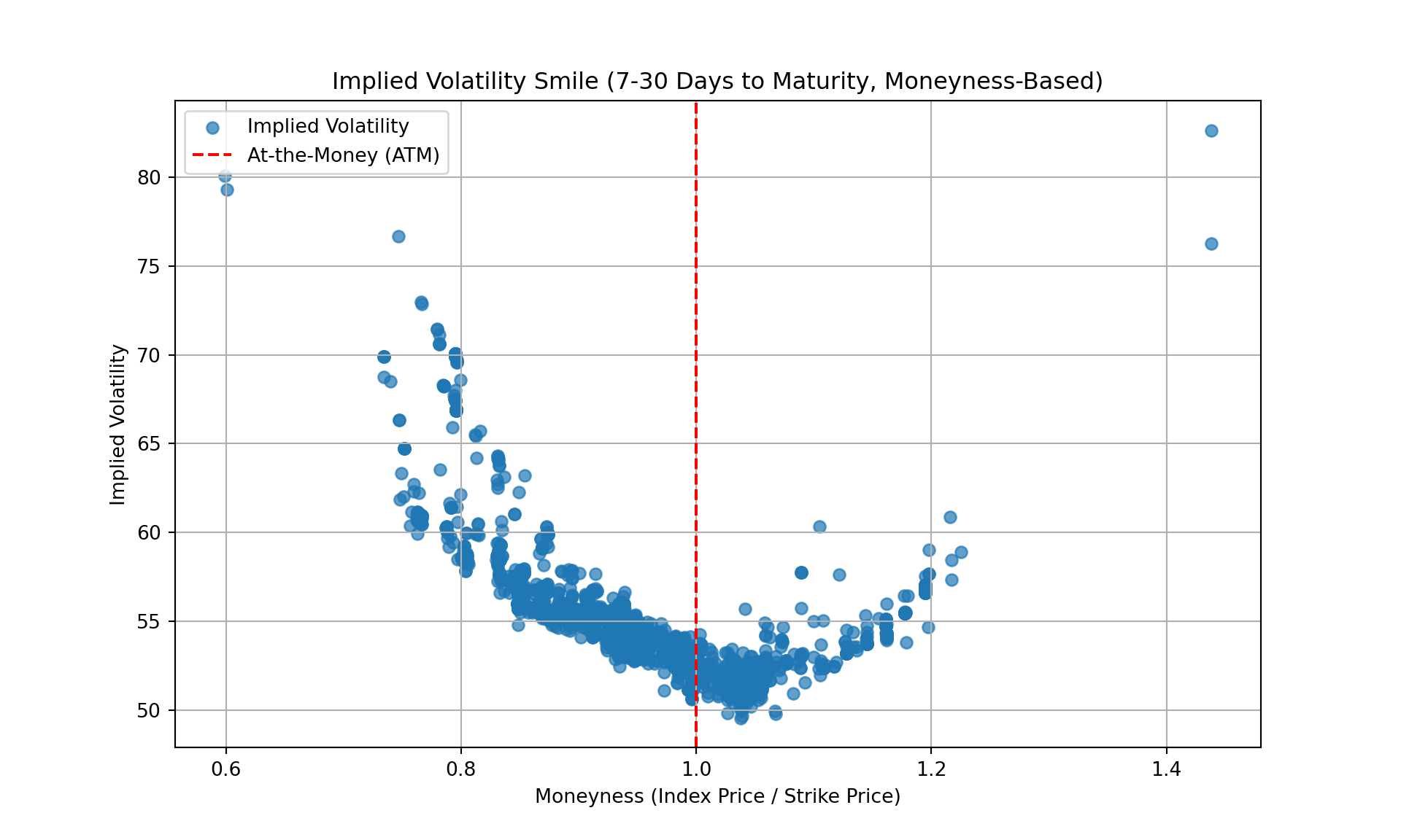
The implied volatility provided by Deribit is derived directly from live market data and reflects the collective sentiment, supply-demand dynamics, and real-time risk perceptions of market participants, without the fridge assumptions of the Black Scholes Formula. This makes it a highly reliable and actionable measure, as it inherently accounts for factors that models like Black-Scholes cannot capture, such as market skewness, kurtosis, and stochastic volatility.

By using Deribit’s IV, we can focus on applying this market-driven insight to strategies like delta hedging, rather than spending time troubleshooting computational issues or compensating for the limitations of traditional models.

Model Deribit Implied Volatility

Lets try to create a model that would forecast the implied volatility of Deribit, using as inputs the characteristics of the option. This model should be non parametric as we dont know what specific model what used by Deribit.

To use the Random Forest model for predicting implied volatility (IV), replacing the analytical Black-Scholes-based calculation, we follow these steps:

1. Filter and Clean the Data:
   • We remove outlier trades that might distort IV (e.g., combo trades, block trades, liquidation events).
   • Clean and engineer features such as moneyness, days to maturity, historical volatility, and moving averages.
   • Ensure no missing or invalid values remain in the features or target (iv).
2. Train a Random Forest Model:
   • We use relevant features that are correlated with IV, such as days_to_maturity, moneyness, and volatility indicators.
   • Train the Random Forest model to predict the IV (target = 'iv') using a training set.
3. Predict IV for the Dataset:
   • We use the trained model to predict IV for the entire dataset or a test set, then replace the calculated IVs in the dataset with the predicted values for further analysis.
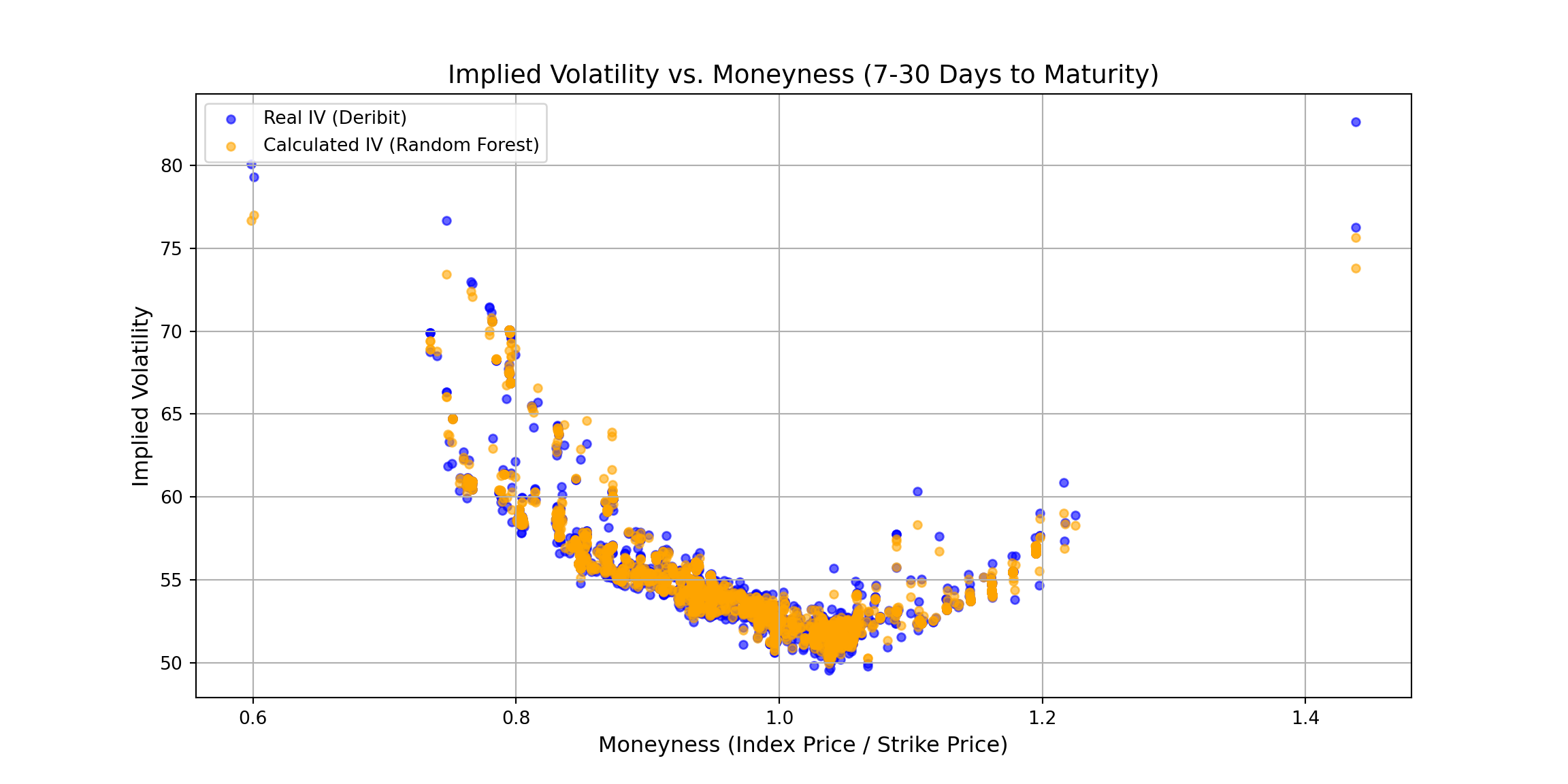
4. Visualize the Volatility Smile:
   • We plot the predicted IVs against the strike prices to observe the smile pattern.

Step-by-Step Code

1. Data Preparation

Start by ensuring your data is clean and ready for modeling.

# Filter trades with valid IV and prices
df = historical_trades.copy()
df['maturity'] = pd.to_datetime(df['maturity'], errors='coerce')
df['timestamp'] = pd.to_datetime(df['timestamp'], errors='coerce')

# Drop rows with invalid dates
df = df.dropna(subset=['maturity', 'timestamp'])

# Calculate days to maturity
df['days_to_maturity'] = (df['maturity'] - df['timestamp']).dt.days
df['time_to_maturity'] = df['maturity'] - df['timestamp']

# Filter out invalid IV values and zero index prices
df = df[(df['iv'] > 0) & (df['iv'] < 500)]
df = df[df['index_price'] > 0]

# Create the 'moneyness' column
df['moneyness'] = df['index_price'] / df['strike']

# Extract the hour of the trade
df['hour'] = df['timestamp'].dt.hour

# Ensure non-negative days to maturity
df['days_to_maturity'] = df['days_to_maturity'].apply(lambda x: max(0, x))

# Sort by timestamp and set as index for rolling calculations
df = df.sort_values('timestamp')
df = df.set_index('timestamp')



# Calculate historical volatility and moving averages
df['historical_volatility'] = df['index_price'].rolling('1h').std() / df['index_price'].rolling(window='1h').mean()
df['moving_average'] = df['index_price'] / df['index_price'].rolling('1h').mean()
df['historical_volatility_7'] = df['index_price'].rolling('7h').std() / df['index_price'].rolling(window='7h').mean()
df['moving_average_7'] = df['index_price'] / df['index_price'].rolling('7h').mean()

# Calculate 3-hour rolling metrics
df['historical_volatility_3'] = df['index_price'].rolling(window='3h').std() / df['index_price'].rolling('3h').mean()
df['moving_average_3'] = df['index_price'] / df['index_price'].rolling('3h').mean()

# Reset the index after rolling calculations
df = df.reset_index()

# Drop rows with NaN values after rolling
df = df.dropna(subset=['historical_volatility', 'moving_average', 'historical_volatility_3', 'moving_average_3'])

# Engineer additional features: minutes to maturity and time to maturity in years
df['minutes_to_maturity'] = df['time_to_maturity'].dt.total_seconds() / 60
df = df[df['minutes_to_maturity'] > 0]  # Remove rows with non-positive maturity
df['time_to_maturity_year'] = df['minutes_to_maturity'] / (365 * 24 * 60)

# Verify final DataFrame
print(f"Data size after all calculations: {len(df)}")

## Data size after all calculations: 4772

print(df[['moneyness', 'historical_volatility', 'historical_volatility_3', 'moving_average', 'moving_average_3']].head())

##    moneyness  historical_volatility  ...  moving_average  moving_average_3
## 1   0.934902               0.000415  ...        1.000293          1.000293
## 2   0.997276               0.000353  ...        1.000227          1.000227
## 3   0.959066               0.000345  ...        1.000285          1.000285
## 4   0.959066               0.000325  ...        1.000228          1.000228
## 5   0.831048               0.000292  ...        1.000048          1.000048
## 
## [5 rows x 5 columns]

2. Train the Random Forest Model

Select features and train a Random Forest model.

from sklearn.model_selection import train_test_split
from sklearn.ensemble import RandomForestRegressor
from sklearn.metrics import mean_squared_error

# Select features and target variable
features = df[['days_to_maturity', 'moneyness', 'historical_volatility', 'hour', 
               'moving_average', 'moving_average_3', 'moving_average_7', 
               'historical_volatility_3', 'historical_volatility_7']]
target = df['iv']

# Split data into training and testing sets
X_train, X_test, y_train, y_test = train_test_split(features, target, test_size=0.2, random_state=42)

# Train the Random Forest model
model = RandomForestRegressor(random_state=42)
model.fit(X_train, y_train)

RandomForestRegressor(random_state=42)

RandomForestRegressor(random_state=42)

# Predict and evaluate
y_pred = model.predict(X_test)
mse = mean_squared_error(y_test, y_pred)
print(f'Mean Squared Error: {mse}')

## Mean Squared Error: 11.621701853968593

3. Predict IV for the Full Dataset

Use the trained model to predict IV for the entire dataset.

# Predict implied volatility for the entire dataset
df['predicted_iv'] = model.predict(features)

4. Visualize the Implied Volatility Smile

Create a plot of predicted IVs against strike prices.

import matplotlib.pyplot as plt

# Filter dataset for options with 7 to 30 days to maturity
filtered_df = df[(df['days_to_maturity'] >= 7) & (df['days_to_maturity'] <= 30)].dropna(subset=['iv', 'moneyness', 'historical_volatility'])

# Plot IV against moneyness
plt.figure(figsize=(12, 6))
plt.scatter(filtered_df['moneyness'], filtered_df['iv'], color='blue', alpha=0.6, label='Real IV (Deribit)', s=20)
plt.scatter(filtered_df['moneyness'], filtered_df['predicted_iv'], color='orange', alpha=0.6, label='Calculated IV (Random Forest)', s=20)

# Add plot titles and labels
plt.title("Implied Volatility vs. Moneyness (7-30 Days to Maturity)", fontsize=14)
plt.xlabel("Moneyness (Index Price / Strike Price)", fontsize=12)
plt.ylabel("Implied Volatility", fontsize=12)
plt.grid(True)
plt.legend()

# Show the plot
plt.show()

5. (Optional) Feature Importance

Analyze which features are most important in predicting IV.

import numpy as np
import matplotlib.pyplot as plt

# Get feature importance
importances = model.feature_importances_
feature_names = features.columns

# Sort features by importance
sorted_indices = np.argsort(importances)[::-1]  # Sort in descending order
sorted_feature_names = feature_names[sorted_indices]
sorted_importances = importances[sorted_indices]

# Plot feature importance
plt.figure(figsize=(10, 6))
plt.barh(sorted_feature_names, sorted_importances, color='skyblue')
plt.xlabel("Importance")
plt.ylabel("Feature")
plt.title("Feature Importance in Predicting IV")
plt.gca().invert_yaxis()  # Invert y-axis to show the highest importance at the top
plt.show()

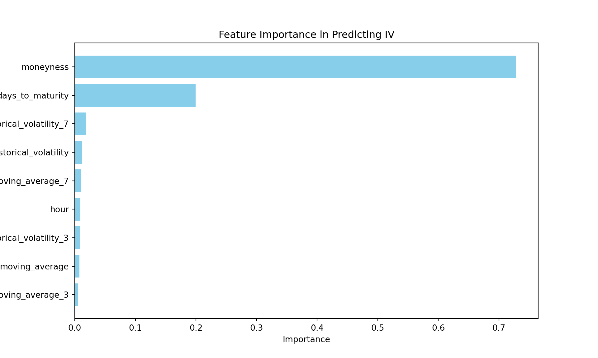
Key Points

• Why Random Forest?: It is a fast, flexible and powerful model that can capture non-linear relationships between features and the target (IV). This is useful since implied volatility may not follow a simple analytical formula.
• Feature Selection: Ensure that the selected features are relevant and clean to avoid introducing noise into the model.
• Interpretability: Use feature importance to understand which variables are driving the model’s predictions.

This approach replaces the analytical Black-Scholes calculation with a data-driven machine learning model to estimate implied volatility. With a bigger data, the random forest could be better trained and more complex models could be made.

Part 3: Implementing a Delta Strategy

What is Delta in Options Trading?

Delta is a measure of how sensitive an option’s price is to changes in the price of the underlying asset. Specifically, for call options, delta represents the expected change in the option’s price for a \1 change in the underlying asset’s price, assuming all other factors remain constant. Mathematically, delta ($\Delta$) is expressed as:

$$ \Delta = \frac{\partial C}{\partial S} $$

Where:

• $C$: Option price
• $S$: Price of the underlying asset

For call options, delta values range between 0 and 1. A delta of 0.5, for instance, means the option’s price is expected to change by \0.50 for every \1 change in the asset’s price. In the case of put options, delta values range between -1 and 0.

Delta also provides insight into the likelihood of the option expiring in the money (ITM). For example, a call option with a delta of 0.7 suggests a 70% chance of the option being ITM at expiration. Delta evolves dynamically based on factors like the underlying asset’s price, time to maturity, and volatility.

Understanding delta is crucial for constructing hedging strategies, as it allows traders to adjust their positions to manage risk effectively.

Code:

# Delta calculation
def calculate_delta(S, K, T, r, sigma):
    d1 = (np.log(S / K) + (r + 0.5 * sigma ** 2) * T) / (sigma * np.sqrt(T))
    return norm.cdf(d1)

# Example: Hedging with 1 option
delta = calculate_delta(S, K, T, r, sigma)
hedge_position = -delta  # Short this fraction of BTC
print(f"Delta Position: {hedge_position} BTC")

## Delta Position: -0.39629035723658007 BTC

Understanding Delta and Using it as a Market Signal

Delta evolves dynamically based on the option’s moneyness, time to maturity, and the volatility of the underlying asset. For example:

• At-the-Money (ATM): Delta is approximately 0.5.
• Out-of-the-Money (OTM): Delta approaches 0 as the option becomes less sensitive to price changes.
• In-the-Money (ITM): Delta approaches 1, reflecting greater sensitivity.

By observing changes in delta, traders can infer shifts in the market sentiment and adjust their positions to maximize profits. For instance, when delta increases significantly, it may signal bullish momentum, while a sharp decrease may indicate bearish trends. Delta-based signals can also help traders decide when to buy or sell Bitcoin to align with market conditions effectively.

Strategy: Using Bitcoin Call Options Delta as a Market Signal

One potential strategy involves monitoring the delta of Bitcoin call options to generate buy/sell signals for Bitcoin itself. Here’s how it works:

1. Set-Up:

   • Use a predictive model (e.g., Random Forest) to estimate implied volatility (IV).
   • Calculate delta for a specific call option, ensuring it is near the current Bitcoin price (ATM) with moderate time to maturity (e.g., 7–30 days).

2. Signal Generation:

   • Buy Signal: When delta increases significantly ($ $ approaches 1), it may indicate bullish momentum in Bitcoin or future bullish expectation. Buy/sell Bitcoin to benefit from potential upward price movement.
   • Sell Signal: When delta decreases sharply ($ $ approaches 0), it may indicate bearish momentum or a future expected fall in price. Sell/buy Bitcoin to avoid potential losses.

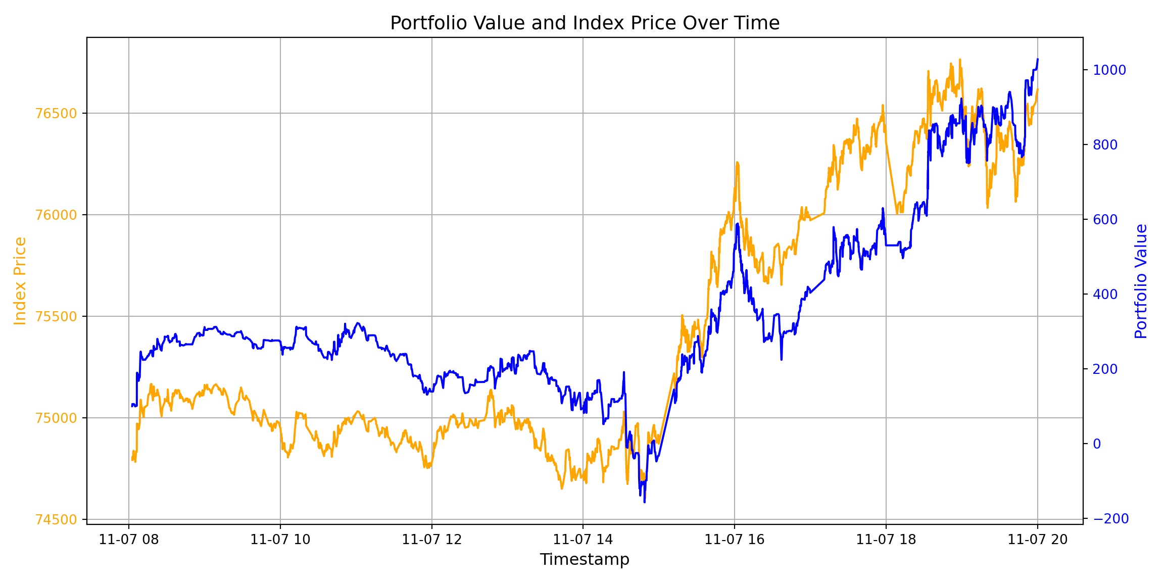
   Our portfolio value would look like this:

$$ P_{t+1} = 100 + D_{t}(S_{t+1} - S_t) + \dots + D_1(S_2 - S_1) $$

Where:

• Initial Cash: The portfolio starts with \100.
• Delta ( $D_t $): Represents the sensitivity of the option’s price to changes in the underlying asset’s price at time t.
• Stock Price Change ($ S_{t+1} - S_t $): The difference in the underlying asset’s price between time t and t+1.

3. Execution:
   • Adjust the trading position based on delta movements while considering transaction costs and rebalancing thresholds to minimize unnecessary trades.

• At every round t, we adjust the portfolio value by buying/selling $D_t * S_{t}$, which would modify the value of our portfolio at t+1 to $ D_t * (S_{t+1} - S_t)$ . This is the core of our strategy, and its succes would depend of updating the value of $ D_t $ at every round t, which at the same time, would be a function of the forecasted implied volatility, as well as the strike price and time to maturity.

Ensuring that $ D_t $ accurately reflects the option’s sensitivity at each time step is crucial.

While the standard way of thinking about options is using the underlying asset’s price $ S_{t}$, for the execution of this strategy, its not the price of the asset that matters, but the delta of the option.

Considering this, $ S_{t}$ in our strategy could be the initial amount of cash of our portfolio. In the first round, as we buy Bitcoin with the whole amount of cash, the value of our portfolio remains unchanged.

4. Risk Management:
   • Use stop-loss orders to limit losses in case of sharp adverse movements.
   • Combine delta signals with other indicators (e.g., volatility or moving averages) to enhance decision-making.

This approach provides a practical and dynamic way to leverage options pricing as a tool for directional trading in Bitcoin markets, making delta a valuable market signal for maximizing profitability.

Workflow for Delta Strategy with Random Forest IV

1. Delta strategy Logic:
   • Adjust the stock position dynamically to match the delta of the option (IV forecasted using the Random Forest model).
   • Track portfolio value, cash position, and transaction costs over time.
2. Simulate Portfolio Performance:
   • Simulate the performance of the portfolio as you hedge delta over time.
3. Plot Results:
   • Visualize key metrics like the portfolio value over time or transaction costs.

df.iterrows()

## <generator object DataFrame.iterrows at 0x15ac4fab0>

Code

import pandas as pd
import matplotlib.pyplot as plt

# Define the delta hedging function
def delta_hedging(df, forecast_iv_column, initial_stock_price, r=0.01, trading_fee_rate=0.002):
    # Initialize portfolio and stock positions
    portfolio_value = 0
    cash_position = initial_stock_price  # Starting with cash equal to initial stock price
    stock_position = 0  # Starting with no stock initially
    
    results = []

    for index, row in df.iterrows():
        S = row['index_price']
        K = row['strike']
        T = row['days_to_maturity'] / 365  # Convert days to years
        date = row['date']
        #print(K)
        sigma_forecast = row[forecast_iv_column] / 100  # Convert percentage to decimal
        
        # Calculate forecasted delta
        delta_forecast = (calculate_delta(S, K, T, r, sigma_forecast))*(-1) #is negative because we are shorting the call
       
        # Calculate the number of stocks to buy/sell to adjust to the new delta
        delta_change = delta_forecast - stock_position
        transaction_cost = 0
        
        if delta_change != 0:
            # Calculate transaction cost: trading fee + network fee
            trading_fee = abs(delta_change) * S * trading_fee_rate
            #transaction_cost = trading_fee + network_fee*S
            transaction_cost = 0
            
            if abs(delta_change * S) > transaction_cost:
                # Update cash position considering transaction cost
                cash_position -= transaction_cost #we substract the transaction cost from the cash position
                
                # Adjust stock position to maintain delta neutrality
                cash_position += delta_change * S #if delta_change is positive, we are buying stock, if negative we are selling stock.
                #If we buy stock, we substract the stock price from the cash position
                stock_position = delta_forecast #we set the stock position to the forecasted delta
                
        
        # Calculate actual option price using Black-Scholes
        #option_price_actual = black_scholes_call(S, K, T, r, sigma_actual)
        
        # Update portfolio value
        portfolio_value = (stock_position * S*(-1)) + cash_position #portfolio value is the stock position times the stock price plus the cash position
        
        # Store results
        results.append({
            'timestamp': row['timestamp'],  # Ensure timestamp exists
            'portfolio_value': portfolio_value,
            'index_price': S
        })
    
    return pd.DataFrame(results)

# Apply delta hedging strategy to the data
df['date']= df['timestamp'].dt.date
results = delta_hedging(df, 'predicted_iv', initial_stock_price=100)

## <string>:3: RuntimeWarning: divide by zero encountered in scalar divide

# Create a dual-axis plot
fig, ax1 = plt.subplots(figsize=(12, 6))

# Left y-axis: Index Price
ax1.plot(results['timestamp'], results['index_price'], label='Index Price', color='orange')
ax1.set_xlabel("Timestamp", fontsize=12)
ax1.set_ylabel("Index Price", fontsize=12, color='orange')
ax1.tick_params(axis='y', labelcolor='orange')
ax1.grid(True)

# Right y-axis: Portfolio Value
ax2 = ax1.twinx()
ax2.plot(results['timestamp'], results['portfolio_value'], label='Portfolio Value', color='blue')
ax2.set_ylabel("Portfolio Value", fontsize=12, color='blue')
ax2.tick_params(axis='y', labelcolor='blue')

# Title
plt.title("Portfolio Value and Index Price Over Time", fontsize=14)

# Show the plot
fig.tight_layout()
plt.show()

Explanation

1. Delta Calculation:
   • The forecasted delta is calculated using the predicted implied volatility (predicted_iv) from the Random Forest model.
2. Portfolio Adjustments:
   • Adjust stock positions dynamically to match the forecasted delta, considering transaction costs.
3. Visualization:
   • Portfolio Value: Track the total portfolio value over time to assess the effectiveness of the strategy.
   • Transaction Costs: Plot cumulative transaction costs to understand the costs
   • Delta Changes: Analyze the frequency and magnitude of adjustments required to maintain the delta strategy.

Key Points

• Accuracy of IV Forecast: The results will depend heavily on the quality of the forecasted IVs (predicted_iv).
• Transaction Costs: Including realistic transaction costs provides a more accurate simulation of the strategy’s performance.
• Further Analysis: You can experiment with different time intervals (e.g., rebalancing daily or hourly) to evaluate how often the portfolio should be adjusted.

Delta as a Market Signal and its Impact on the Portfolio

In this approach, the portfolio value is influenced by the deltas of all traded call options, acting as a market signal. Delta behaves like a weighted sum: it is low for out-of-the-money options, high for at-the-money options, and particularly significant for options with high volatility and short days to maturity. Longer-dated options are less impactful due to their lower weight.

Delta dynamically adjusts based on the option’s moneyness and time to maturity. For deep out-of-the-money options, delta approaches 0, limiting losses if the price drops. Conversely, for deep in-the-money options, delta nears 1, amplifying gains if the price rises. Shorter time to maturity further sharpens delta changes, making the portfolio more sensitive to price fluctuations when at-the-money.

While this demonstrates the potential for strategic delta adjustments, the intention of this blog is not to define a trading strategy but to explore delta’s role in portfolio dynamics.

Posible modeling of delta?

It could be possible to model delta, though this would not be followed in this blog, i will write the ideas: Variables that affects $ D_i $:

$$ D_i = \Phi(d_1), \quad \text{where } d_1 = \frac{\ln(S/K) + (r + \sigma^2 / 2)T}{\sigma \sqrt{T}} $$

Where:

• Stock Price ($S$): As $S$ increases, $d_1$ increases, and so does $(d_1)$ . A higher $S$ leads to a higher delta for a call option, amplifying the positive impact of $S_{i+1} - S_i$ on the portfolio.
• Strike Price ( $K$ ): A lower K (deep in-the-money option) increases $ d_1 $, leading to a higher delta. If the option starts in the money, delta is closer to 1, and the portfolio becomes more sensitive to price changes.
• Time to Maturity ( T ): As T decreases, $\sqrt{T}$ decreases, which can increase $d_1 $ (depending on the relationship between $S/K$ and $\sigma $). However, as $T $ , delta converges to 1 if the option is in the money and to 0 if it is out of the money.
• Volatility ( $\sigma$ ): Higher volatility increases $ d_1$ when $ S/K > 1 $, leading to a higher delta. In volatile markets, delta can change more significantly, affecting the portfolio positively or negatively depending on the price direction.

Cumulative Sum

$$ \sum_{i=1}^{t} D_i(S_{i+1} - S_i) $$

The overall portfolio value is the sum of all $D_i(S_{i+1} - S_i) $ terms. Each term is influenced by: • Consistency of Positive Movements: If most $ S_{i+1} - S_i > 0$ , and delta $D_i$ is positive, the sum of these terms will increase $P_{t+1}$ . • Magnitude of Delta: The magnitude of $D_i$ amplifies or dampens the effect of $S_{i+1} - S_i$ . Higher delta (closer to 1) leads to greater sensitivity to price changes, increasing the portfolio’s reaction to upward movements.

Considering the implications of normal distribution between the stock price, we could try to use non parametric modeling, like i talked about it this post in the blog.

Conclusion

In this blog, we embarked on a journey through the world of Bitcoin options, using tools and strategies that bridge finance, data science, and machine learning. Let’s summarize what we achieved and the tools that made it possible:

Key Takeaways:

1. Data Collection with the Deribit API:

   • We demonstrated how to use the Deribit API to fetch historical Bitcoin options data efficiently.
   • By automating the data retrieval process in Python, we handled the complexities of time-interval-based queries, ensuring well-structured datasets ready for analysis.

2. Understanding the Black-Scholes Model:

   • The blog provided a clear and simplified explanation of the Black-Scholes formula, a cornerstone of options pricing in finance.
   • We explored implied volatility, its significance in market sentiment, and limitations of the Black-Scholes model, enhancing the understanding of real-world market dynamics.

3. Applying Machine Learning for Forecasting:

   • By employing a Random Forest model, we showcased a modern approach to predict implied volatility from market data.
   • This non-parametric method allowed us to move beyond traditional assumptions and adapt to complex, real-world patterns in options trading.

4. Delta Strategy for Portfolio Management:

   • We implemented a delta strategy, adjusting stock positions dynamically based on the delta of Bitcoin options.
   • Through visualization and simulation, we highlighted how delta can act as a market signal and a tool for risk management in financial portfolios.