Kernel Density and Local Estimators with Confidence Bands
Exploring nonparametric methods for density and regression estimation
Introduction
In this post, we’ll explore Kernel Density Estimation (KDE), Local Constant Estimator, and Local Linear Estimator. Additionally, we’ll introduce 95% Confidence Bands (both point-wise and universal) to quantify the uncertainty in the estimators.
This will provide a more complete understanding of these non-parametric methods and how to use them effectively.
Kernel Density Estimation (KDE) with Confidence Bands
Kernel Density Estimation (KDE) estimates the probability density function of a random variable by smoothing data points with a kernel function. To evaluate the reliability of the KDE, we add point-wise and universal confidence bands.
Kernel Density Estimation (KDE): Theory and Application
Kernel Density Estimation (KDE) is a non-parametric method used to estimate the probability density function (PDF) of a dataset. Unlike parametric approaches, KDE does not assume the data follows a specific distribution (e.g., normal distribution). Instead, it constructs the density estimate by smoothing individual data points using a kernel function. This makes KDE highly flexible and particularly useful when the underlying data distribution is unknown or non-standard, such as in financial data where heavy tails and skewness are common.
The KDE is defined as:
$$ \hat{f}(x) = \frac{1}{n h} \sum_{i=1}^n K\left(\frac{x - X_i}{h}\right), $$
where:
- $ \hat{f}(x) $ is the estimated density at point $ x $,
- $ X_i $ are the data points,
- $ K $ is the kernel function (e.g., Epanechnikov or Gaussian),
- $ h $ is the bandwidth, controlling the smoothness of the estimate.
The choice of bandwidth $ h $ is crucial. Smaller $ h $ values lead to a more flexible estimate but can result in overfitting, while larger $ h $ values produce a smoother density at the cost of losing detail.
When to Use KDE
KDE is particularly valuable in situations where the density of the data is unknown and may deviate from standard distributions. For example:
- Exploratory Analysis: When we want to visualize the shape of the data’s distribution without assuming normality.
- Non-Normal Data: Financial data, for instance, often exhibit heavy tails or skewness, making KDE a robust choice to uncover the true density.
In the code example above, the KDE is compared to a normal density estimation.
Confidence Bands
Confidence bands, both pointwise and uniform, provide uncertainty estimates for the density function:
- Pointwise Confidence Bands quantify the variability at specific points, showing how confident we are about the estimate at each ( x ).
- Uniform Confidence Bands cover the entire range of ( x ), ensuring that the true density lies within the band with a given probability.
These bands help evaluate the reliability of the KDE and highlight areas where the estimate may be less accurate due to data sparsity or noise.
Example: KDE with Confidence Bands
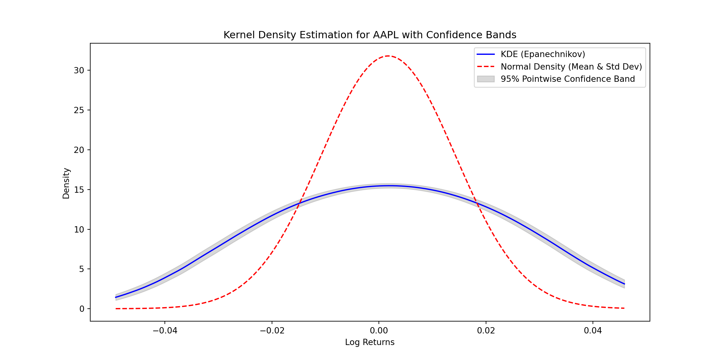
Here’s a KDE estimator example with pointwise confidence bands for financial data using the Epanechnikov kernel. The code downloads stock price data (APPLE), computes log returns, and estimates the density with confidence bands. The normal density is also calculated for comparison. :
import numpy as np
import matplotlib.pyplot as plt
from scipy.stats import norm
import yfinance as yf

# Download financial data
def download_financial_data(ticker, start_date, end_date):
    data = yf.download(ticker, start=start_date, end=end_date)
    log_returns = np.log(data['Close'] / data['Close'].shift(1)).dropna()
    return log_returns

# Define KDE with Epanechnikov Kernel
def epanechnikov_kernel(u):
    return np.where(np.abs(u) <= np.sqrt(5), (3 / (4 * np.sqrt(5))) * (1 - u**2 / 5), 0)

def kernel_density_estimate(x_values, data, bandwidth):
    densities = np.zeros_like(x_values)
    for i, x in enumerate(x_values):
        weights = epanechnikov_kernel((x - data) / bandwidth)
        densities[i] = np.sum(weights) / (len(data) * bandwidth)
    return densities

# Function to calculate variance estimate for pointwise confidence intervals
def variance_estimate(x_values, data, bandwidth):
    n = len(data)
    variances = np.zeros_like(x_values)
    for i, x0 in enumerate(x_values):
        K_h_values = epanechnikov_kernel((data - x0) / bandwidth) / bandwidth
        term1 = (1 / n) * np.sum(K_h_values**2)
        term2 = ((1 / n) * np.sum(K_h_values))**2
        variances[i] = (term1 - term2) / n
    return variances

# Function to calculate the normal density
def normal_density_estimate(x_values, mean, std_dev):
    return (1 / (np.sqrt(2 * np.pi * std_dev**2))) * np.exp(-((x_values - mean)**2) / (2 * std_dev**2))

# Download and preprocess financial data
ticker = "AAPL"  # Example ticker
start_date = "2023-01-01"
end_date = "2024-01-01"
log_returns = download_financial_data(ticker, start_date, end_date)
## /Users/luisj/anaconda3/lib/python3.11/site-packages/yfinance/utils.py:775: FutureWarning: The 'unit' keyword in TimedeltaIndex construction is deprecated and will be removed in a future version. Use pd.to_timedelta instead.
##   df.index += _pd.TimedeltaIndex(dst_error_hours, 'h')
##
[*********************100%%**********************]  1 of 1 completed
# KDE and confidence bands
x_values = np.linspace(log_returns.min(), log_returns.max(), 1000)
bandwidth = 0.02  # Example bandwidth
density_estimates = kernel_density_estimate(x_values, log_returns.values, bandwidth)

# Pointwise confidence bands
alpha = 0.05
variance_estimates = variance_estimate(x_values, log_returns.values, bandwidth)
z_alpha = norm.ppf(1 - alpha / 2)
lower_bounds = density_estimates - z_alpha * np.sqrt(variance_estimates)
upper_bounds = density_estimates + z_alpha * np.sqrt(variance_estimates)

# Normal density for comparison
mean_returns = log_returns.mean()
std_returns = log_returns.std()
normal_density = normal_density_estimate(x_values, mean_returns, std_returns)

# Plot results
plt.figure(figsize=(12, 6))
plt.plot(x_values, density_estimates, label="KDE (Epanechnikov)", color='blue')
plt.plot(x_values, normal_density, label="Normal Density (Mean & Std Dev)", color='red', linestyle='--')
plt.fill_between(x_values, lower_bounds, upper_bounds, color='gray', alpha=0.3, label="95% Pointwise Confidence Band")
plt.xlabel("Log Returns")
plt.ylabel("Density")
plt.title(f"Kernel Density Estimation for {ticker} with Confidence Bands")
plt.legend()
plt.show()
Explanation:
- Epanechnikov Kernel: The function smooths the data points based on the Epanechnikov formula. A bandwidth parameter controls the degree of smoothing.
- Normal Density: The normal density estimate is calculated using the sample mean and standard deviation for comparison with the KDE.
- Confidence Bands:
- Variance Estimate: Variance for pointwise confidence intervals is computed based on kernel weights.
Conclusion
KDE is a powerful tool for density estimation, especially when the underlying distribution of the data is unknown or non-standard. It is particularly useful in domains like finance, where data often deviate from normality, exhibiting heavy tails or irregular shapes. By using kernels and bandwidths, KDE provides a flexible, data-driven approach to estimate densities without relying on strict parametric assumptions. The addition of confidence bands further enhances its utility by quantifying the uncertainty in the estimates, making KDE a robust choice for both exploratory and confirmatory data analysis.
Introduction: Nonparametric Regression
Using the estimation of Kernel Density Estimators, now we can approach the expected values of Y given X (using the esitmated density). By doing this, we can obtain non parametric estimators. Nonparametric regression methods are powerful tools for estimating the relationship between a response variable $ Y $ and a predictor $ X $, without assuming a specific parametric form for the underlying relationship. Unlike traditional linear or polynomial regression, nonparametric methods adapt to the data’s structure, providing flexibility in modeling complex relationships.
Two widely used nonparametric regression estimators are the Nadaraya-Watson Estimator and the Local Linear Estimator. While both methods use kernel functions to assign weights to data points based on their proximity to the evaluation point, they differ in how they model the local behavior of the data.
The Nadaraya-Watson Estimator
The Nadaraya-Watson Estimator is a simple, kernel-based approach to regression. For a given point $x $, the estimator computes the weighted average of the response variable $ Y $ using the weights determined by the kernel function:
$$ \hat{m}(x) = \frac{\sum_{i=1}^n K_h(x - X_i) Y_i}{\sum_{i=1}^n K_h(x - X_i)}, $$
where:
- $( K_h(u) = \frac{1}{h} K\left(\frac{u}{h}\right) ) $ is the kernel function scaled by the bandwidth ( h ),
- $( X_i )$ and $( Y_i )$ are the predictor and response variables, respectively.
The kernel function ( K ) determines the weight assigned to each observation. Common kernels include the Gaussian kernel and the Epanechnikov kernel. The bandwidth ( h ) controls the smoothness of the estimate: smaller values of ( h ) result in a more flexible, less smooth fit, while larger values yield smoother estimates.
While the Nadaraya-Watson Estimator is simple and effective, it can suffer from boundary bias. Near the edges of the data, the kernel weights become asymmetric, leading to inaccuracies in the estimated values.
The Local Linear Estimator
The Local Linear Estimator extends the Nadaraya-Watson approach by fitting a local linear regression in the neighborhood of each evaluation point ( x ). Instead of assuming a constant value for ( Y ) (as in NW), this method models ( Y ) as a linear function:
$$ Y \approx \theta_0 + \theta_1 (X - x).$$
For a given ( x ), the parameters $ \theta_0 $ and $ \theta_1 $ are estimated by minimizing a kernel-weighted least-squares objective:
$$ \min_{\theta_0, \theta_1} \sum_{i=1}^n K_h(X_i - x) \left[ Y_i - \theta_0 - \theta_1 (X_i - x) \right]^2. $$
The solution gives the local linear regression coefficients $ \hat{\theta}_0 $ and $ \hat{\theta}_1 $, and the estimator at ( x ) is $ \hat{m}(x) = \hat{\theta}_0 $.
By allowing for a linear fit within the kernel window, the Local Linear Estimator addresses the boundary bias issue present in the Nadaraya-Watson Estimator. It can better capture the local structure of the data and typically performs well both near the edges and in regions with varying density.
Comparison of the Two Methods
| Feature | Nadaraya-Watson Estimator | Local Linear Estimator |
|---|---|---|
| Model Assumption | Locally constant | Locally linear |
| Bias near boundaries | High (prone to boundary bias) | Low (reduces boundary bias) |
| Complexity | Simple (weighted average) | More complex (weighted least squares) |
| Behavior near edges | Underestimates or overestimates response | Handles boundaries more accurately |
Both methods depend heavily on the choice of the kernel function and the bandwidth parameter, which control the smoothness and flexibility of the estimates.
Python Code
import numpy as np
import matplotlib.pyplot as plt
from scipy.stats import norm
from scipy.integrate import quad

# Define kernels
def epanechnikov_kernel(u):
    return np.where(np.abs(u) <= np.sqrt(5), (3 / (4 * np.sqrt(5))) * (1 - u**2 / 5), 0)

# Nadaraya-Watson Estimator
def nadaraya_watson(X, Y, x_grid, bandwidth, kernel=epanechnikov_kernel):
    estimates = []
    for x in x_grid:
        weights = kernel((X - x) / bandwidth)
        numerator = np.sum(weights * Y)
        denominator = np.sum(weights)
        estimates.append(numerator / denominator if denominator > 0 else 0)
    return np.array(estimates)

# Local Linear Estimator
def local_linear_estimator(X, Y, x_eval, bandwidth, kernel=epanechnikov_kernel):
    n = len(X)
    U = np.vstack([np.ones(n), X - x_eval]).T
    W = np.diag(kernel((X - x_eval) / bandwidth) / bandwidth)
    theta_hat = np.linalg.inv(U.T @ W @ U) @ (U.T @ W @ Y)
    return theta_hat[0], theta_hat[1]

# Variance estimator for pointwise confidence intervals
def compute_s_hat(X, residuals, x_eval, bandwidth, kernel=epanechnikov_kernel):
    weights = kernel((X - x_eval) / bandwidth) / bandwidth
    weights_squared = weights**2
    residuals_squared = residuals**2
    f_hat = np.sum(weights) / (len(X) * bandwidth)
    s_hat = np.sqrt(np.sum(weights_squared * residuals_squared) / (len(X)**2 * f_hat**2))
    return s_hat

# Generate synthetic data
np.random.seed(42)
X = np.linspace(0, 10, 100)
Y = np.sin(X) + np.random.normal(0, 0.2, size=len(X))

# Define evaluation grid and bandwidth
x_grid = np.linspace(0, 10, 200)
bandwidth = 0.8

# Estimate Nadaraya-Watson
nw_estimates = nadaraya_watson(X, Y, x_grid, bandwidth)

# Estimate Local Linear
ll_intercepts = []
for x in x_grid:
    intercept, _ = local_linear_estimator(X, Y, x, bandwidth)
    ll_intercepts.append(intercept)

# Residuals for Nadaraya-Watson
nw_residuals = Y - nadaraya_watson(X, Y, X, bandwidth)

# Pointwise Confidence Intervals
alpha = 0.05
z_alpha = norm.ppf(1 - alpha / 2)
pointwise_lower = []
pointwise_upper = []
s_hat_values = []

for x_eval, m_eval in zip(x_grid, nw_estimates):
    s_hat = compute_s_hat(X, nw_residuals, x_eval, bandwidth)
    s_hat_values.append(s_hat)
    pointwise_lower.append(m_eval - z_alpha * s_hat)
    pointwise_upper.append(m_eval + z_alpha * s_hat)

# Plot Nadaraya-Watson with Pointwise CI
plt.figure(figsize=(12, 6))
## <Figure size 1200x600 with 0 Axes>
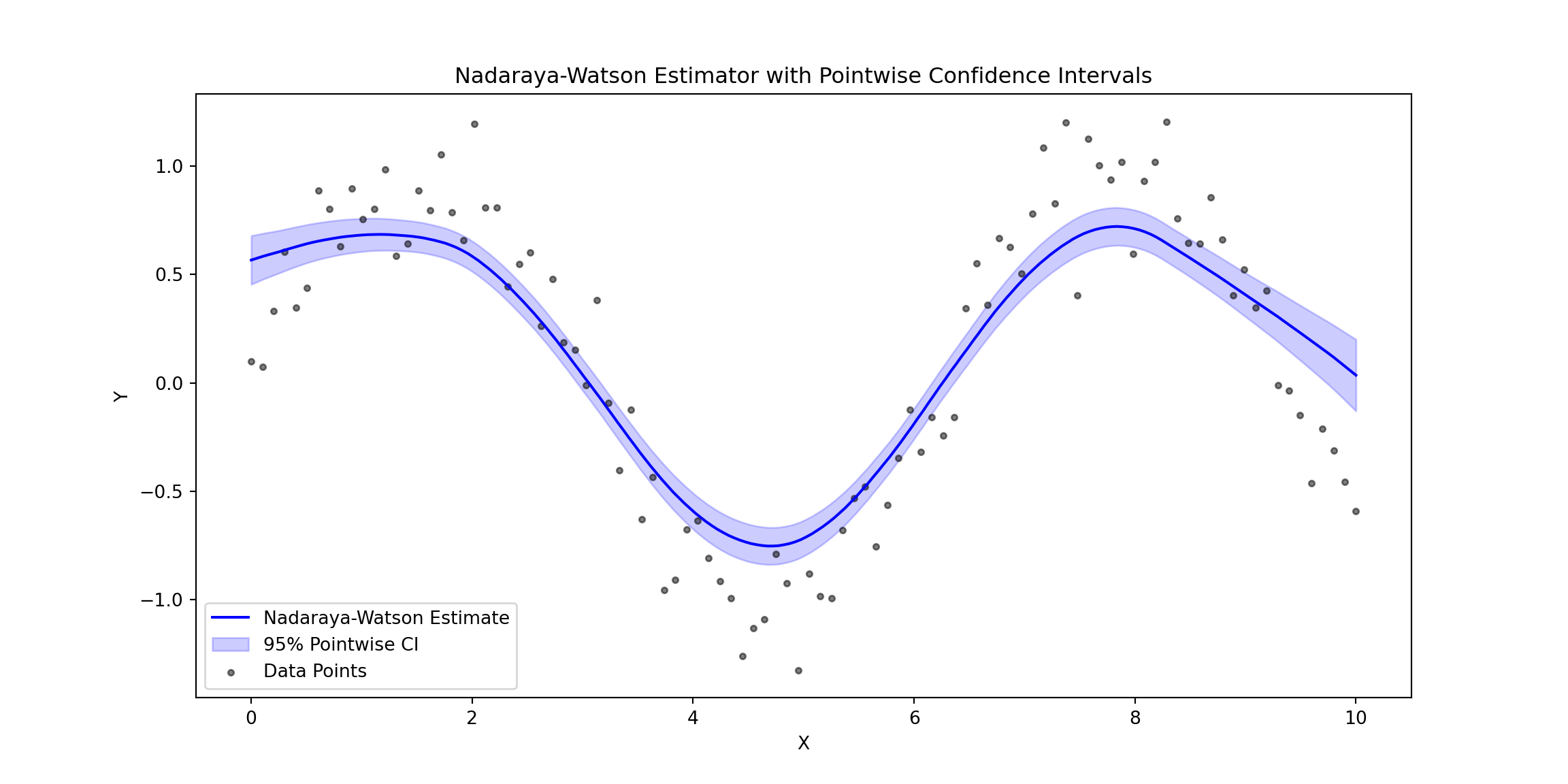
plt.plot(x_grid, nw_estimates, label="Nadaraya-Watson Estimate", color="blue")
## [<matplotlib.lines.Line2D object at 0x17d060550>]
plt.fill_between(x_grid, pointwise_lower, pointwise_upper, color="blue", alpha=0.2, label="95% Pointwise CI")
## <matplotlib.collections.PolyCollection object at 0x17d0f1b90>
plt.scatter(X, Y, alpha=0.5, label="Data Points", color="black", s=10)
## <matplotlib.collections.PathCollection object at 0x17d0e6cd0>
plt.title("Nadaraya-Watson Estimator with Pointwise Confidence Intervals")
## Text(0.5, 1.0, 'Nadaraya-Watson Estimator with Pointwise Confidence Intervals')
plt.xlabel("X")
## Text(0.5, 0, 'X')
plt.ylabel("Y")
## Text(0, 0.5, 'Y')
plt.legend()
## <matplotlib.legend.Legend object at 0x17d069d10>
plt.show()
# Uniform Confidence Bands
def compute_G(x_grid, X, residuals, bandwidth, kernel=epanechnikov_kernel):
    n = len(X)
    G_values = []
    for x_eval in x_grid:
        kernel_values = kernel((X - x_eval) / bandwidth) / bandwidth
        total_weight = np.sum(kernel_values)
        weights = kernel_values / total_weight if total_weight > 0 else np.zeros_like(kernel_values)
        xi = np.random.normal(0, 1, n)
        s_hat = compute_s_hat(X, residuals, x_eval, bandwidth)
        G_x = np.sum(xi * residuals * weights / s_hat)
        G_values.append(G_x)
    return np.array(G_values)

def gaussian_multiplier_bootstrap(x_grid, X, residuals, bandwidth, kernel=epanechnikov_kernel, B=1000, alpha=0.05):
    bootstrap_sup = []
    for _ in range(B):
        G_values = compute_G(x_grid, X, residuals, bandwidth, kernel)
        bootstrap_sup.append(np.max(np.abs(G_values)))
    return np.quantile(bootstrap_sup, 1 - alpha)

q_alpha = gaussian_multiplier_bootstrap(x_grid, X, nw_residuals, bandwidth)
uniform_lower = nw_estimates - q_alpha * np.array(s_hat_values)
uniform_upper = nw_estimates + q_alpha * np.array(s_hat_values)

# Plot with Uniform Confidence Bands
plt.figure(figsize=(12, 6))
## <Figure size 1200x600 with 0 Axes>
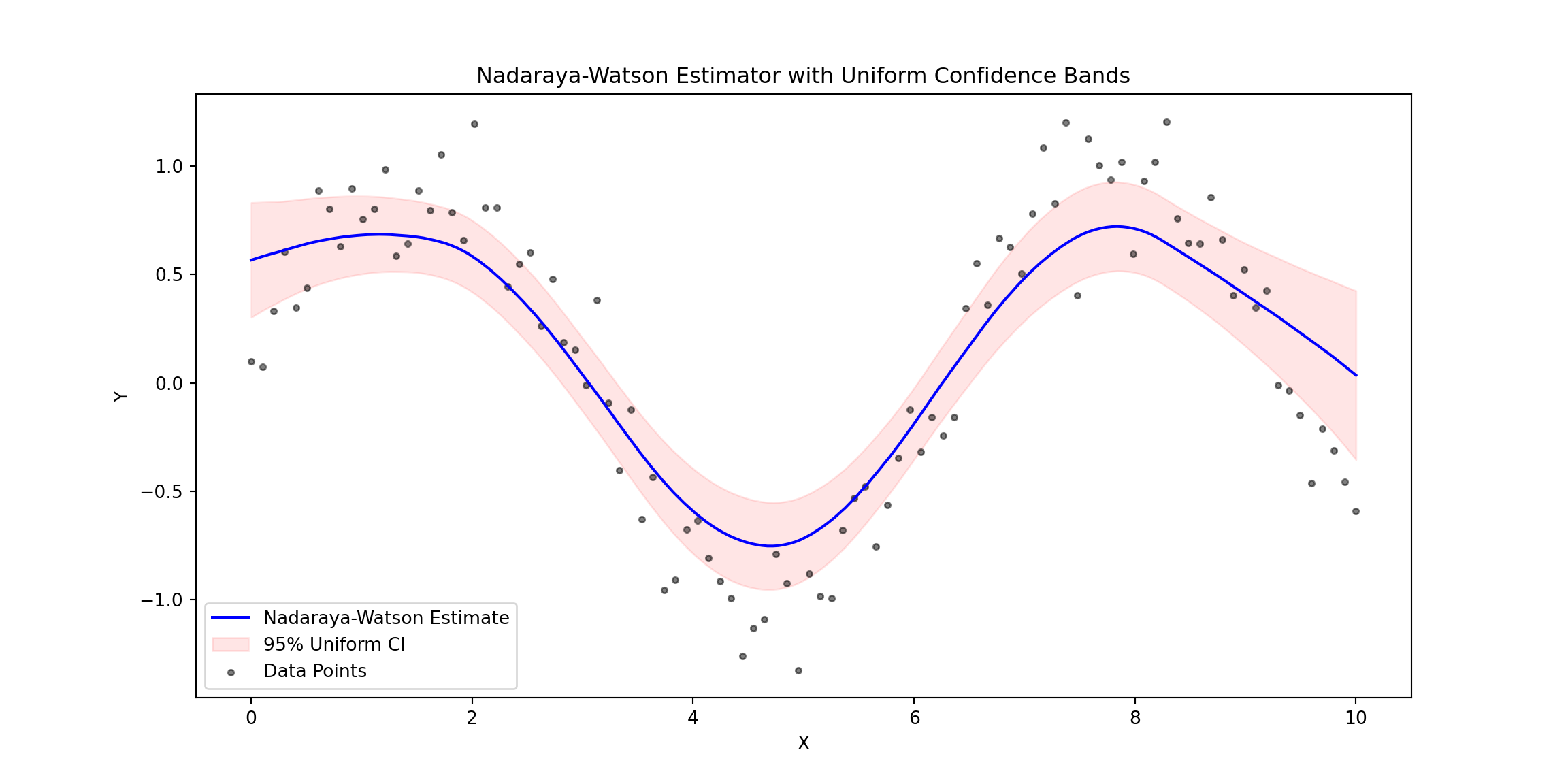
plt.plot(x_grid, nw_estimates, label="Nadaraya-Watson Estimate", color="blue")
## [<matplotlib.lines.Line2D object at 0x17de5ebd0>]
plt.fill_between(x_grid, uniform_lower, uniform_upper, color="red", alpha=0.1, label="95% Uniform CI")
## <matplotlib.collections.PolyCollection object at 0x17de92590>
plt.scatter(X, Y, alpha=0.5, label="Data Points", color="black", s=10)
## <matplotlib.collections.PathCollection object at 0x17de2c410>
plt.title("Nadaraya-Watson Estimator with Uniform Confidence Bands")
## Text(0.5, 1.0, 'Nadaraya-Watson Estimator with Uniform Confidence Bands')
plt.xlabel("X")
## Text(0.5, 0, 'X')
plt.ylabel("Y")
## Text(0, 0.5, 'Y')
plt.legend()
## <matplotlib.legend.Legend object at 0x17de9ee90>
plt.show()
Pointwise vs. Uniform Confidence Bands
Pointwise and uniform confidence bands both quantify the uncertainty in regression estimates but differ in their scope. Pointwise confidence bands provide an interval estimate for the regression function at each specific point ( x ), indicating the range where the true function is likely to lie with a given probability (e.g., 95%). However, these intervals do not account for the simultaneous uncertainty across all points in the domain.
In contrast, uniform confidence bands account for the entire range of ( x ), ensuring that the true regression function lies within the band at all points with a specified probability (e.g., 95%). While pointwise bands are narrower and easier to compute, uniform bands are more conservative and robust, capturing the overall uncertainty across the entire function.
Key Features
- Synthetic Data: Non-linear function $ Y = \sin(X) + \text{noise} $.
- Nadaraya-Watson Estimation: Smoothed estimates with Epanechnikov kernel.
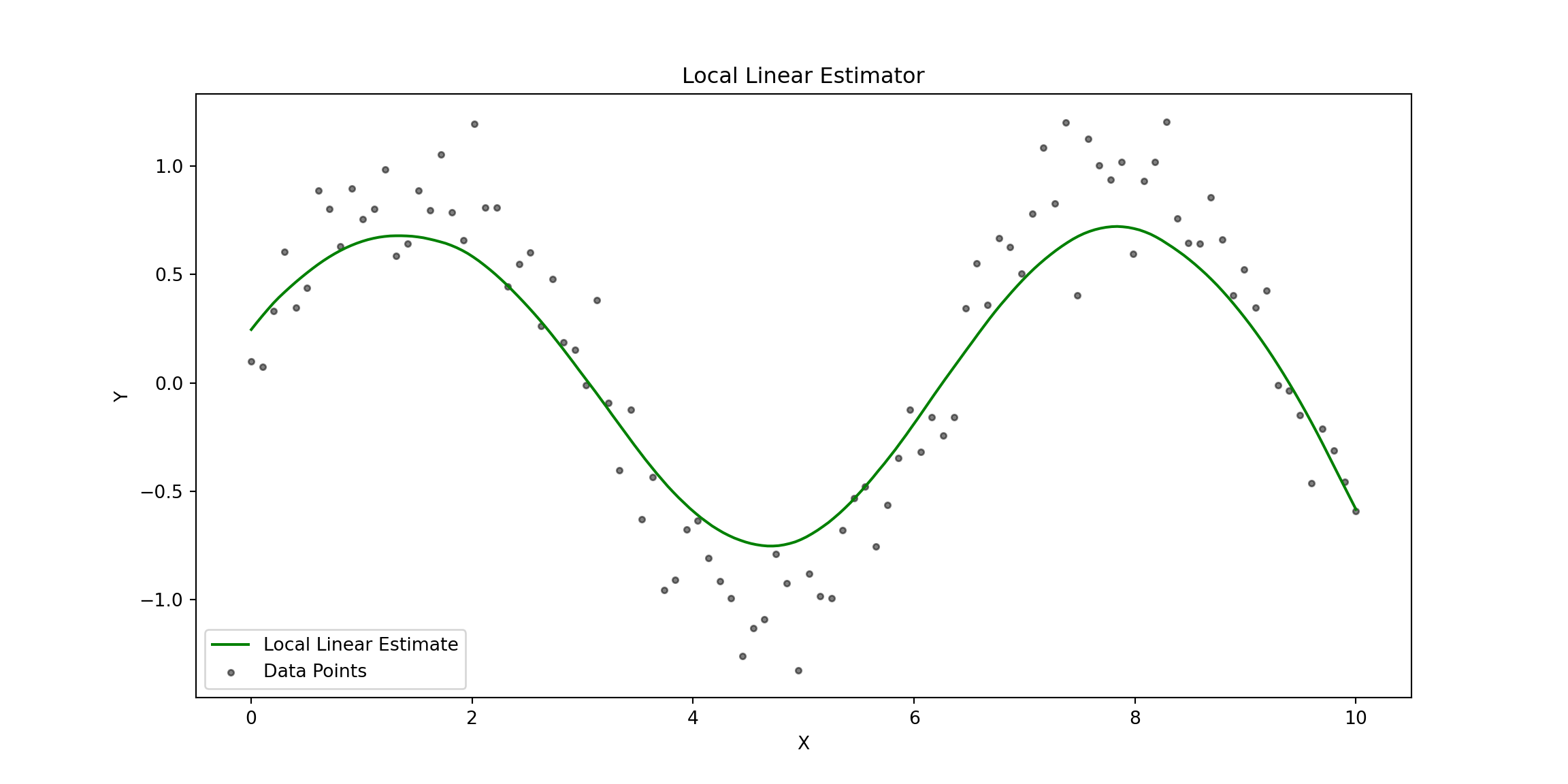
- Local Linear Estimation: Estimates the function with reduced bias.
- Pointwise Confidence Intervals: Calculated using the standard error of residuals.
- Uniform Confidence Bands: Computed via Gaussian multiplier bootstrap.
This approach demonstrates the application of kernel-based regression estimators and provides clear visual comparisons of pointwise and uniform confidence intervals.
# Plot Local Linear Estimator
plt.figure(figsize=(12, 6))
## <Figure size 1200x600 with 0 Axes>
plt.plot(x_grid, ll_intercepts, label="Local Linear Estimate", color="green")
## [<matplotlib.lines.Line2D object at 0x17ded4890>]
plt.scatter(X, Y, alpha=0.5, label="Data Points", color="black", s=10)
## <matplotlib.collections.PathCollection object at 0x17dec5990>
plt.title("Local Linear Estimator")
## Text(0.5, 1.0, 'Local Linear Estimator')
plt.xlabel("X")
## Text(0.5, 0, 'X')
plt.ylabel("Y")
## Text(0, 0.5, 'Y')
plt.legend()
## <matplotlib.legend.Legend object at 0x17ded64d0>
plt.show()
# Plot Comparison: Nadaraya-Watson vs Local Linear Estimators
plt.figure(figsize=(12, 6))
## <Figure size 1200x600 with 0 Axes>
plt.plot(x_grid, nw_estimates, label="Nadaraya-Watson Estimate", color="blue")
## [<matplotlib.lines.Line2D object at 0x17dec8590>]
plt.plot(x_grid, ll_intercepts, label="Local Linear Estimate", color="green", linestyle="--")
## [<matplotlib.lines.Line2D object at 0x17deabfd0>]
plt.scatter(X, Y, alpha=0.5, label="Data Points", color="black", s=10)
## <matplotlib.collections.PathCollection object at 0x17dec4290>
plt.title("Comparison: Nadaraya-Watson vs Local Linear Estimators")
## Text(0.5, 1.0, 'Comparison: Nadaraya-Watson vs Local Linear Estimators')
plt.xlabel("X")
## Text(0.5, 0, 'X')
plt.ylabel("Y")
## Text(0, 0.5, 'Y')
plt.legend()
## <matplotlib.legend.Legend object at 0x17de7f210>
plt.show()
Conclusion
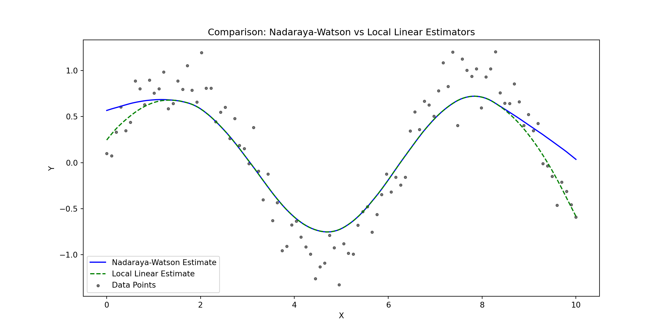
The plot compares the Nadaraya-Watson Estimator (solid blue line) and the Local Linear Estimator (dashed green line) against the observed data points (gray dots). Here are some key observations:
Overall Fit:
- Both estimators capture the non-linear structure of the data effectively, reflecting the sinusoidal trend of the underlying function.
- The estimators generally align well in regions where the data density is higher.
Boundary Behavior:
- At the edges of the data (e.g., near $ X = 0 $ and $ X = 10 $), the Nadaraya-Watson Estimator shows a stronger bias, curving upward or downward.
- The Local Linear Estimator performs better at the boundaries, maintaining a smoother and more accurate extrapolation due to its local linear adjustment.
Flexibility vs. Bias:
- The Nadaraya-Watson Estimator, being locally constant, is slightly less responsive to rapid changes in the data, particularly at the boundaries where it suffers from higher bias.
- The Local Linear Estimator, with its linear adjustment, is better equipped to handle such variations, leading to reduced bias and improved accuracy near the edges.
Central Region:
- In the central region of the domain (e.g., between $ X = 3 $ and $ X = 7 $), both estimators perform similarly, as the data density is sufficient for accurate local smoothing.
Practical Implications:
- The Nadaraya-Watson Estimator may be more suitable for datasets where boundary effects are not a concern and the goal is simplicity, or we are unsure of the linear assumptions in the data. Its locally constant approach avoids making strong assumptions about the underlying structure, making it a safer choice for exploratory analysis in small datasets
- The Local Linear Estimator is preferable when boundary accuracy is critical or when the data exhibits sharp trends that require more adaptive modeling.It can handle variations better, especially when there is enough data to justify the assumption of local linearity.
Final Conclusion
In this post, we explored the theory and implementation of Kernel Density Estimation (KDE), the Nadaraya-Watson Estimator, and the Local Linear Estimator, along with methods to construct 95% confidence bands (pointwise and uniform). These non-parametric techniques provide a flexible framework for analyzing data without assuming a specific parametric model, making them powerful tools for understanding complex relationships.
Kernel Density Estimation (KDE) allows us to estimate the probability density function of a variable, with the kernel function and bandwidth playing key roles in balancing bias and variance. The inclusion of confidence bands helps quantify the uncertainty in the density estimates, providing deeper insights into the reliability of the results.
The Nadaraya-Watson Estimator is a simple and intuitive approach to nonparametric regression that uses kernel-weighted averages to estimate the response variable. While effective in capturing trends, it is susceptible to boundary bias and less responsive to sharp changes in the data.
The Local Linear Estimator, on the other hand, fits a locally linear model to reduce bias at the boundaries and adapt better to variations in the data. Its ability to handle local trends makes it a more robust choice in many scenarios, especially when data density varies across the domain.
Confidence bands enhance these methods by providing uncertainty estimates. Pointwise confidence bands quantify uncertainty at individual points, while uniform confidence bands ensure coverage over the entire domain, offering a more robust perspective on the estimator’s reliability.
The Nadaraya-Watson Estimator is particularly useful for exploratory analysis, especially with small datasets or when there are uncertainties about the linearity of the underlying relationships. In contrast, the Local Linear Estimator is better suited for situations where accuracy near boundaries or sharp data trends is critical.
In conclusion, these nonparametric methods offer flexibility and adaptability in data analysis, making them essential tools for uncovering complex patterns and relationships. By carefully selecting the appropriate estimator, kernel function, and bandwidth, you can tailor these approaches to meet your analytical objectives effectively.
Luis José Zapata Bobadilla
Economist - Analyst
Economist and advocate for innovative digital payment systems. Passionate about exploring monetary policy, blockchain technology, machine learning, and their transformative impact on the financial ecosystem.