Introduction

Have you ever wondered how a government might evaluate the impact of a new scholarship program that only kicks in when a student’s GPA exceeds a specific threshold? Or how a policy change affecting tax rates for households above a certain income level actually influences economic behavior? These are just a couple of scenarios where Regression Discontinuity Design (RDD) comes into play—a powerful tool for causal inference when treatment assignment hinges on a cutoff.

In this blog post, we’ll explore RDD by building a local linear regression from the ground up—no magic packages or black-box functions here! Instead, we’ll simulate data that features a clear jump at a predetermined cutoff and then walk through the entire estimation process step by step. You’ll see exactly how the treatment effect is estimated right at the threshold and how the confidence interval is constructed to quantify uncertainty.

By starting from zero, we aim to demystify the inner workings of RDD, ensuring that you not only learn how to implement it but also understand the underlying logic behind the method. Whether you’re evaluating educational policies, economic interventions, or any scenario with a clear threshold effect, this hands-on guide is your first step toward mastering RDD.

Regression Discontinuity Design (RDD) is a quasi-experimental method used to estimate causal effects when treatment assignment is determined by a cutoff in a continuous variable (the running variable). The key idea is that units just below and just above the cutoff are very similar, so a jump in the outcome at the cutoff can be interpreted as the causal effect of the treatment.

Mathematically, let $$ m(x) = E[Y \mid X=x] $$

be the conditional expectation of the outcome Y given the running variable X. Suppose that there is a discontinuity at x = c so that: $$ m(x) = \begin{cases} m_0(x), & x < c, \newline m_1(x), & x \ge c. \end{cases} $$ The treatment effect at the cutoff is then estimated as: $$ \hat{\tau} = m_1(c) - m_0(c). $$

The variance of the estimated effect is: $$ \operatorname{Var}(\hat{\tau}) = \operatorname{Var}(m_1(c)) + \operatorname{Var}(m_0(c)) $$

and the 95% confidence interval (CI) is given by: $$ \hat{\tau} \pm z_{0.025} \sqrt{\operatorname{Var}(m_1(c)) + \operatorname{Var}(m_0(c))} $$ with $ z_{0.025} \approx 1.96$.

In the following sections, we illustrate these concepts with a simulated dataset.

1. Simulated Data

We simulate a dataset with 500 observations. The running variable x is drawn uniformly from [-10,10]. The outcome y is generated with a discontinuity (a jump) at x=0. In our simulation, for x < 0 we set: $$ y = 5 + 0.3x + \varepsilon, $$ and for $x \ge 0$: $$ y = 7 + 0.3x + \varepsilon, $$ with$\varepsilon \sim N(0,1)$.

import numpy as np
import pandas as pd

# Set the seed for reproducibility
np.random.seed(42)

# Simulate 500 observations for the running variable x
N = 500
x = np.random.uniform(-10, 10, size=N)

# Generate noise
error = np.random.normal(0, 1, size=N)

# Generate outcome y with a jump at x = 0 (jump of 2 units)
y = np.where(x < 0, 5 + 0.3 * x, 7 + 0.3 * x) + error

# Create a DataFrame
data = pd.DataFrame({'x': x, 'y': y})
print(data.head())

##           x          y
## 0 -2.509198   4.588997
## 1  9.014286  11.580457
## 2  4.639879   9.342387
## 3  1.973170   7.015047
## 4 -6.879627   2.037697

In this simulated example, the cutoff is at $x=0$.

2. Epanechnikov Kernel

The Epanechnikov kernel is used to assign weights to observations based on their distance from the cutoff. Observations closer to the cutoff are given higher weights. The kernel is defined as: $$ K(u) = \begin{cases} 0.75 (1 - u^2) & \text{if } |u| \le 1, \newline 0 & \text{otherwise.} \end{cases} $$ This topic is explained more deeply on my other blog post about Kernel Density Estimation.

def epanechnikov_kernel(u):
    """
    Epanechnikov kernel function.
    
    Returns:
    K(u) = 0.75 * (1 - u^2) for |u| <= 1, and 0 otherwise.
    """
    if abs(u) <= 1:
        return 0.75 * (1 - u**2)
    else:
        return 0

3. Local Linear Regression

To estimate the outcome function on either side of the cutoff, we perform a weighted linear regression. We center the running variable at the cutoff $c=0$ so that: $$ x_{\text{centered}} = x - c = x. $$ The local linear regression model is: $$ y = \beta_0 + \beta_1 x_{\text{centered}} + \varepsilon. $$ At $x_{\text{centered}} = 0$, the predicted outcome is $\beta_0$, which estimates m(c).

def local_linear_regression(df, y_variable, x_variable, cutoff, bandwidth, kernel_function):
    """
    Performs local linear regression on observations below and above the cutoff.
    
    The running variable is centered at the cutoff:
    $$ x_{centered} = x - c $$
    so that the intercept represents the estimated outcome at the cutoff, i.e., $$ m(c) = \\beta_0 $$.
    """
    df_local = df.copy()
    # Center the running variable at the cutoff (c = 0)
    df_local['x_centered'] = df_local[x_variable] - cutoff
    df_local['constant'] = 1

    # Compute kernel weights based on the scaled distance from the cutoff
    df_local['weights'] = df_local['x_centered'].apply(lambda x: kernel_function(x / bandwidth))
    
    # Split data into observations below and above the cutoff
    df_below = df_local[df_local['x_centered'] <= 0]
    df_above = df_local[df_local['x_centered'] > 0]
    
    def _weighted_regression(sub_df, y_var):
        if sub_df.empty:
            return np.array([np.nan, np.nan]), np.full((2, 2), np.nan)
        X = sub_df[['constant', 'x_centered']].values
        Y = sub_df[y_var].values
        W = np.diag(sub_df['weights'].values)
        try:
            XTWX_inv = np.linalg.inv(X.T @ W @ X)
            theta = XTWX_inv @ (X.T @ W @ Y)
            residuals = Y - X @ theta
            variance_matrix = XTWX_inv @ (X.T @ W @ np.diag(residuals**2) @ W @ X) @ XTWX_inv
        except np.linalg.LinAlgError:
            return np.array([np.nan, np.nan]), np.full((2, 2), np.nan)
        return theta, variance_matrix
    
    theta_below, var_below = _weighted_regression(df_below, y_variable)
    theta_above, var_above = _weighted_regression(df_above, y_variable)
    return theta_below, var_below, theta_above, var_above

4. RDD Estimator

The RDD estimator computes the treatment effect as the difference in the predicted outcomes at the cutoff: $$ \hat{\tau} = \hat{m}_1(0) - \hat{m}_0(0), $$ where $\hat{m}_1(0)$ and $\hat{m}_0(0)$ are the intercepts from the regressions above and below the cutoff, respectively. The variance of the treatment effect is: $$ \operatorname{Var}(\hat{\tau}) = \operatorname{Var}(\hat{m}_1(0)) + \operatorname{Var}(\hat{m}_0(0)), $$ and its standard error is the square root of this sum.

def rdd_estimator(df, y_variable, x_variable, cutoff, bandwidth, kernel_function):
    """
    Estimates the RDD treatment effect as the difference in the predicted outcome at the cutoff.
    
    Since the running variable is centered at the cutoff,
    the predicted outcome is simply the intercept:
    $$ \\hat{m}(c) = \\beta_0. $$
    Thus, the treatment effect is:
    $$ \\hat{\\tau} = \\hat{m}_1(c) - \\hat{m}_0(c). $$
    """
    theta_below, var_below, theta_above, var_above = local_linear_regression(
        df, y_variable, x_variable, cutoff, bandwidth, kernel_function)
    
    if np.any(np.isnan(theta_below)) or np.any(np.isnan(theta_above)):
         return np.nan, np.nan
    
    # Predicted outcome at the cutoff is the intercept (when x_centered = 0)
    pred_below = theta_below[0]
    pred_above = theta_above[0]
    treatment_effect = pred_above - pred_below
    
    # Variance of the intercept estimates (using the selector vector e0 = [1, 0])
    e0 = np.array([1.0, 0.0])
    se = np.sqrt(e0 @ (var_below + var_above) @ e0)
    
    return treatment_effect, se

5. Running the Analysis and Constructing the Confidence Interval

We now run the RDD estimator using a chosen bandwidth and compute the 95% confidence interval. Recall, the 95% CI is given by: $$ CI_\text{95%} = \hat{\tau} \pm 1.96 \times SE(\hat{\tau}). $$

from scipy.stats import norm
# Choose a bandwidth (experiment with this value)
bandwidth = 2.0

# Run the RDD estimator on the simulated data. Here, the cutoff is 0.
treatment_effect, se = rdd_estimator(data, 'y', 'x', cutoff=0, bandwidth=bandwidth, kernel_function=epanechnikov_kernel)

if not np.isnan(treatment_effect):
    print("RDD Estimate (ATE): {:.4f}".format(treatment_effect))
    print("Standard Error: {:.4f}".format(se))
    
    # Compute the 95% confidence interval.
    alpha = 0.05
    z = norm.ppf(1 - alpha/2)  # Approximately 1.96 for a 95% CI.
    ci_lower = treatment_effect - z * se
    ci_upper = treatment_effect + z * se
    print("95% Confidence Interval: [{:.4f}, {:.4f}]".format(ci_lower, ci_upper))
else:
    print("RDD estimation failed. Please check your data or bandwidth.")

## RDD Estimate (ATE): 1.9539
## Standard Error: 0.3026
## 95% Confidence Interval: [1.3607, 2.5470]

6. Graphical Representation: Plotting the Local Linear Fits and Confidence Intervals

Below we plot the estimated local linear regressions on either side of the cutoff, along with their pointwise 95% confidence intervals.

import matplotlib.pyplot as plt

def plot_rdd_fit(df, y_variable, x_variable, cutoff, bandwidth, kernel_function, n_grid=100, alpha=0.05):
    """
    Plots the local linear regression fits with pointwise 95% confidence intervals.
    
    The regression is estimated separately on each side of the cutoff.
    """
    # Get the estimates from local linear regressions.
    theta_below, var_below, theta_above, var_above = local_linear_regression(df, y_variable, x_variable, cutoff, bandwidth, kernel_function)
    
    if np.any(np.isnan(theta_below)) or np.any(np.isnan(theta_above)):
        print("Local-linear regression failed on one side. No plot produced.")
        return
    
    # Extract coefficients for each side.
    beta0_below, beta1_below = theta_below
    beta0_above, beta1_above = theta_above
    
    # Create grids for values below and above the cutoff.
    x_min, x_max = df[x_variable].min(), df[x_variable].max()
    grid_below = np.linspace(x_min, cutoff, n_grid)
    grid_above = np.linspace(cutoff, x_max, n_grid)
    
    # Compute the z-value for the (1-alpha) CI.
    z_val = norm.ppf(1 - alpha/2)
    
    # Compute predictions and confidence intervals for observations below the cutoff.
    mhat_below = []
    ci_lower_below = []
    ci_upper_below = []
    for xg in grid_below:
        # Prediction: m0(x) = beta0_below + beta1_below * (x - cutoff)
        pred = beta0_below + beta1_below * (xg - cutoff)
        vec = np.array([1.0, xg - cutoff])
        var_pred = vec @ var_below @ vec
        se_pred = np.sqrt(var_pred)
        mhat_below.append(pred)
        ci_lower_below.append(pred - z_val * se_pred)
        ci_upper_below.append(pred + z_val * se_pred)
        
    # Compute predictions and confidence intervals for observations above the cutoff.
    mhat_above = []
    ci_lower_above = []
    ci_upper_above = []
    for xg in grid_above:
        # Prediction: m1(x) = beta0_above + beta1_above * (x - cutoff)
        pred = beta0_above + beta1_above * (xg - cutoff)
        vec = np.array([1.0, xg - cutoff])
        var_pred = vec @ var_above @ vec
        se_pred = np.sqrt(var_pred)
        mhat_above.append(pred)
        ci_lower_above.append(pred - z_val * se_pred)
        ci_upper_above.append(pred + z_val * se_pred)
    
    #Lets create the original lines from the formula
    y_below = 5 + 0.3 * grid_below
    y_above = 7 + 0.3 * grid_above
    
    # Plot the results.
    plt.figure(figsize=(8,6))
    plt.plot(grid_below, mhat_below, color='blue', label=r'$\hat{m}_0(x)$')
    plt.fill_between(grid_below, ci_lower_below, ci_upper_below, color='blue', alpha=0.3)
    plt.plot(grid_above, mhat_above, color='red', label=r'$\hat{m}_1(x)$')
    plt.fill_between(grid_above, ci_lower_above, ci_upper_above, color='red', alpha=0.3)
    plt.axvline(cutoff, color='black', linestyle='--', label='Cutoff')
    plt.xlabel('Running Variable')
    plt.ylabel('Outcome')
    plt.title('Local Linear Regression Fit with 95% Confidence Intervals')
    #Lets also add the original data
    plt.scatter(df[x_variable], df[y_variable], color='black', alpha=0.15, label='Data')
    #Lets plot the original lines
    plt.plot(grid_below, y_below, color='green', label='y = 5 + 0.3x',linestyle='-.')
    plt.plot(grid_above, y_above, color='purple', label='y = 7 + 0.3x',linestyle='-.')
    plt.legend()
    plt.show()

# Call the plotting function.
plot_rdd_fit(data, 'y', 'x', cutoff=0, bandwidth=bandwidth, kernel_function=epanechnikov_kernel)

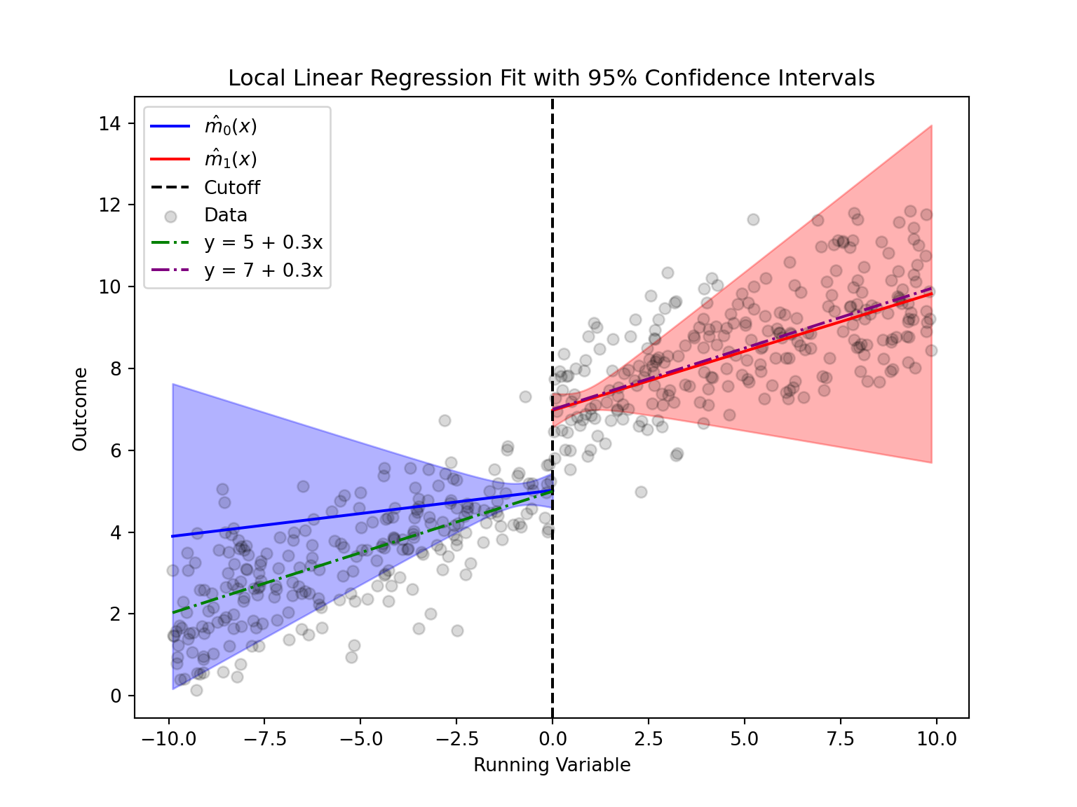
As we can see, the local linear regression effectively emphasizes the data closest to the cutoff by using weighted observations. While the slope estimates may be more variable—since they rely on data closer to the cutoff, the intercept provides a robust estimate of the treatment effect at the cutoff. This is why the confidence interval is narrow near the cutoff (where the model is most precise) and widens as we move away, reflecting that our inference is primarily focused on the discontinuity point. Overall, the model accurately captures the differences in outcomes between the two sides of the cutoff.

Conclusion

In this post we have:

• Simulated data with a discontinuity at $x=0$,
• Used an Epanechnikov kernel to weight observations based on their proximity to the cutoff,
• Performed local linear regressions on each side of the cutoff to estimate the outcome functions, and
• Estimated the treatment effect as the jump at the cutoff, along with its 95% confidence interval.

This example provides a didactic introduction to RDD. By focusing on data near the cutoff, RDD isolates the causal effect of the treatment. Happy coding and exploring RDD!